For example, consider a chart, its top edge is bound to row 1, and its bottom edge is bound to row 13. Similarly, its left edge is bound to column D, and its right edge to column J. That means if you insert a new row between 1 to 13, the whole chart shifts down one row. If you insert a column to the left of column D, the whole chart shifts one column to the right.
Even more interesting is what happens if you insert rows or columns in the area that the chart overlaps. For example, if you insert a new row between the current row 8 and row 9, the chart stretches, becoming one row taller. Similarly, if you delete column E, the chart compresses, becoming one column thinner.
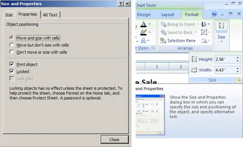
You can change this sizing behavior, first select the chart and head to the ribbon's Chart Tools: Format > Size section. Then, click the dialog launcher (the square-with-an-arrow icon in the bottom-right corner). When the Size and Properties dialog box appears, choose the Properties tab. You'll see three "Object positioning" options. The standard behavior is "Move and size with cells", but you can also create a chart that moves around the worksheet but never resizes itself ("Move but don't size with cells") and a chart that's completely fixed in size and position ("Don't move or size with cells").