
- Setup Criteria Range for Advanced Filter
- Filter Data By The Exact Criteria
- Filter Data by Multiple Criteria
- Using Logical Operators in Advanced Filters
- Filter Data By Formulas
- Use Wildcards in Advanced Filter Criteria
Assuming you have data in a worksheet, and you want to filter it based on specific criteria and copy the results to another location:
First, set up the criteria range: Create a new range in your worksheet or on another worksheet where you will define your filter criteria. Ensure that each column header in this range matches the column header in your list range.
For example, if your data has headers in cells Year, Month, Product, City, and Sales, create a new range with the same headers in another location and fill in the criteria you want to filter by in cells below the headers.
The figure below displays the records that match the criteria range, namely that the Month column has the value January and the City column has the value Boston.
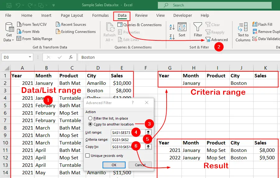
- Select the range of data you want to filter. Make sure that the first row contains column headers.
- Click on the
Datatab and click onAdvancedbutton in theSort & Filtergroup. This will open theAdvanced Filterdialog box. - In the Advanced Filter dialog box under the
Action, choose one of the following options:Filter the list, in place: filters the data in the same location-
Copy to another locationcopies the filtered data to another location, we choose this option.
-
List range: Select the range that you want to filter, by default, Excel automatically fills in the range of your selected data. Criteria range: Select the range that contains your criteria (the range you set up in step 1).Copy to: If you choseCopy to another location, specify the range where you want the filtered results to be displayed.- Click
OK.
Excel will apply the advanced filter based on the criteria you defined, and either filter the data in place or copy the filtered results to the specified location.
Filter Data By The Exact Criteria
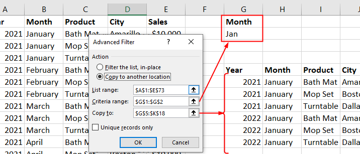
If your criterion is Jan and you perform an Advanced Filter on a long list of names, Excel would show not only the name Jan, but also names such as January, Jangler, Jangle, etc. In other words, any name that begins with the letters Jan, in that order, will be considered a match for the criteria. See the following figure, the Advanced Filter showing the filtered data containing January for the criterion Jan:
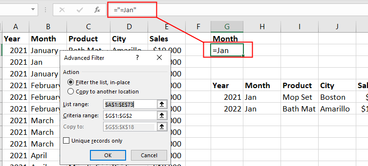
To force Excel to find exact matches e.g., in this case, find only the name Jan enter your criteria as ="=Jan".
Filter Data by Multiple Criteria
One point to keep in mind when using the Advanced Filter is that two or more criteria placed directly underneath the applicable heading use an OR statement:
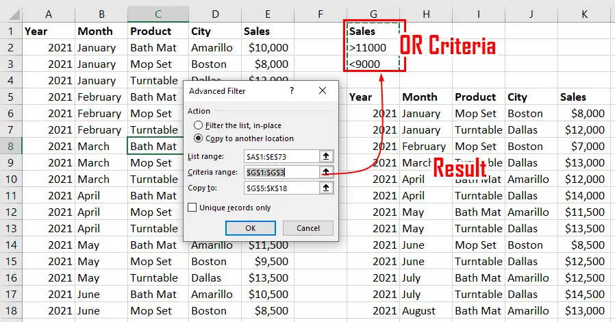
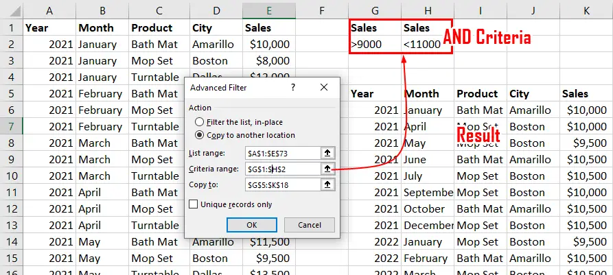
If you want to use an AND statement, the column headings and their criteria must appear twice, side by side. The figure below shows how to use the OR operator to filter your data, and the next figure shows how to use the AND operator.
Using Logical Operators in Advanced Filters
In the criteria range, you can use logical operators like:
=(equal to)<(less than)>(greater than)<=(less than or equal to)>=(greater than or equal to)<>(not equal to)
Here’s an example of how to use logical operators in the criteria range:
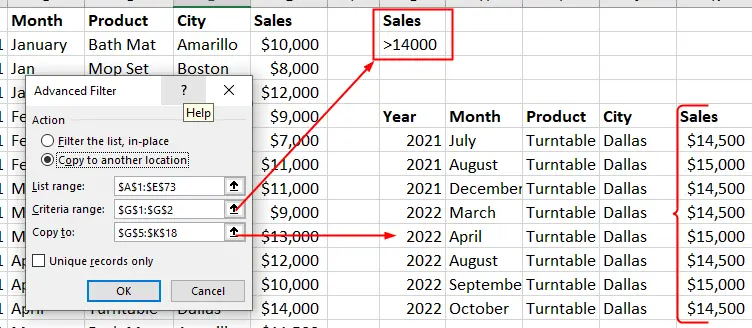
In the above figure, the data is filtered by Sales and only records with sales values greater than 14000 are shown.
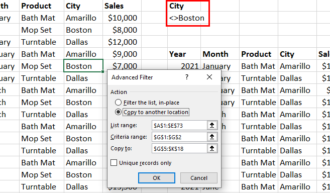
The next example uses the <> (not equal to) operator, for example, if you want to filter the data by their City and exclude those from Boston, you can use the <>Boston criteria to specify the exclusion:
Filter Data By Formulas
It’s important to note that whenever you use a formula for your criteria, you must not use above the criteria a heading that is identical to the one within the table. For example, if you have a list of numeric data in column E (Sales) and the list begins in cell E2 (with E1 being the heading), and you need to extract all the numbers in that list that are greater than the average, you would use criteria such as these:
=E2>AVERAGE($E$2:$E$100)If the criteria were placed in cell G2, the criteria range would be $G$1:$G$2, but $G$1 could not contain the same heading as the one the list uses. It must be either blank or a different heading altogether. See the following figure:
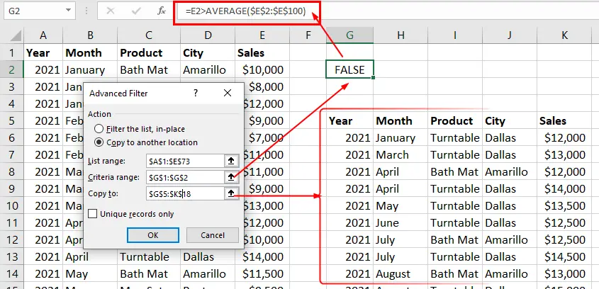
It also is important to note that any formula you use should return either TRUE or FALSE. The range for the average function is made absolute by the addition of dollar signs, while the reference to cell E2 is a relative reference. This is needed because when you apply the Advanced Filter, Excel will see that E2 is a relative reference and will move down the list one entry at a time and return either TRUE or FALSE. If it returns TRUE, it knows it needs to be extracted. If it returns FALSE, it does not meet the criteria; therefore, it will not be shown.
Filter data to extract all the values that appear more than once
Also assume that many of the names are repeated in the range $E$2:E$100, with E1 being the headings. Also, assume that many of the headings are repeated numerous times. You have been given the task of extracting from the list all the names that appear more than once. To do this you need to use the Advanced Filter and the following formula as your criteria:
=COUNTIF($E$2:$E$100,E2)>1Use Wildcards in Advanced Filter Criteria
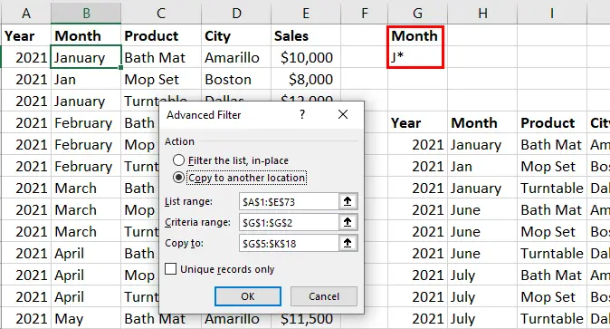
J* matches months started with J.Wildcards help you to to filter data that does not match an exact value, but rather a pattern or a part of a value. For example, you may want to filter all the names that start with A or all the products that contain book. This is where wildcard characters come in handy. Excel supports three wildcard characters:
*(asterisk), represents any number of characters (including no characters). The criteria*ingmatches all the values that end withing. For example,*ingmatches Going, Lying, Coming, Gaming, and so on.?(question mark), represents any single character. The criteriab?tmatches but, bit, bat, bet, bot, and so on.
The criteriaB????filter all the values that have four letters and start withB..~(tilde) is used to escape the other wildcard characters. For example, if you want to filter all the values that contain*(asterisk), you can use the criteria~*.