The two methods you will use are methods we have used in the past when we received an updated copy of a spreadsheet and we needed to identify which cells in the updated copy differed from the ones in the original copy. Both methods save hours of tedious manual checking and, more importantly, eliminate the possibility of mistakes.
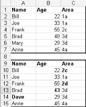
For the following examples, we copied the newer data onto the same sheet as the older data beforehand. Figure below shows how the data is presented as two ranges. Note that for easier viewing, we boldfaced the cells in Table 2 that are not the same as their counterparts in Table 1.
Figure. Two ranges to be compared

Method 1: Using True or False
The first method involves entering a simple formula into another range of the same size and shape. The best part about this method is that you can add the formula in one step without having to copy and paste.
To compare the ranges shown in the figure, select the range E1:G7, starting from cell E1. This ensures that E1 is the active cell in the selection. With this range selected, click in the Formula bar and type the following:
=A1=A9
Enter the preceding formula by pressing Ctrl-Enter at the same time. In doing so, you are entering the relative reference formula into each cell of the selection. This is the standard method of entering a formula into an array of cells and having their references change appropriately.
The range E1:G7 should be filled with True (the same) and False (not the same) values.
If your two sets of data reside on different worksheets, you can use a third worksheet to store the True/False values simply by array-entering the formula. For example, assuming the second table of data is on Sheet2 and starts in cell A9, and the original table of data is on Sheet1 and starts in cell A1, on a third worksheet you can array-enter this formula:
=Sheet1!A1=Sheet2!A9
You might find it useful to adjust your zoom downward when working with large amounts of data.
To delete an array-entered formula, you must select and delete the whole range. You cannot delete part of it.
Method 2: Using Conditional Formatting
The second method is often preferred, as it is easier to make any needed changes once the comparison is made. However, with this method, both sets of data must reside on the same worksheet, which should entail only a simple copy and paste.
Again, assuming we're comparing the preceding two ranges, select the range A1:C7, starting from cell A1. This ensures that A1 is the active cell in the selection.
With this range selected, select Format » Conditional Formatting.... Select Formula Is and then type the following formula:
=NOT(A1=A9)
Click the Format button, shown in the figure, and choose the format with which you want to highlight the differences.
Figure. Conditional formatting dialog

Click OK and all the differences will be formatted according to the format you chose.
When or if you make any changes to your data, the cells' format will automatically revert back to normal if the cell content is the same as the cell in the other table.