When using Excel's database functions, you can specify up to 256 different criteria. You might, for example, want to sum amounts in column A where the corresponding amount in column B is greater than 100 and the corresponding age in column C is less than 40. If, however, you want to sum amounts where corresponding amounts in column B are less than 50, you need to use another function and a different range of criteria. It would much easier if you had a single function and could easily and quickly change the criteria! If you have never used Excel's database functions before, we strongly recommend that you familiarize yourself with them, as they are very good for extracting statistical information from an Excel database or table.
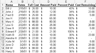
To see how this works, set up your data as shown in Figure. Keep the column headings the same, but the data that resides in it can be any fictitious data. Name this table of data, including all column headings, AllData. Name the sheet Data.
Figure. Proposed data

Insert another worksheet and call this worksheet Results. In cell A2, enter the following formula:
=Data!A1
Copy this across to cell F2 so that you have a mirror image of your table headings. In cell A3, enter any name that exists in your table on the data sheet, such as John D. Then, in cell B3, enter the following formula:
=DGET(AllData,B2,$A$2:$A$3)
Copy this formula across to cell F3 and format cells C3:F3 in the required format.
To quickly copy cells such as this without formatting, select the cell, right-click the fill handle, and, holding down the right mouse button, drag across as far as needed. Then select Fill Without Formatting.
The corresponding data should be extracted out of the table for the name you entered into cell A3. This is just a simple example of how you can use the DGET function to extract relevant information.
If you get the #NUM! error, it means you have two or more identical names in your Name column.
At this point, most people would follow the same concept for all names for which they need information extracted from the table. However, this effort is unnecessary.
As you are always referencing cell A3 for the name, it would make a lot more sense in most cases if you could simply have a drop-down list in cell A3 containing all the names that are in the table. You can use Excel's standard validation feature to create such a list. However, as the original list of names resides on another worksheet, you cannot reference the list in the same way as you would a list residing on the same sheet-i.e., a standard range reference. You can overcome this easily by naming the Name column in the original table, then using that name as the list source for the validation.
As most tables are not static-in other words, data is usually continuously added and removed-you should consider using a dynamic named range for the Names column. See Create Ranges That Expand and Contract for more details on this.
Click back onto the Data sheet and, with any cell selected, select Insert » Name » Define. In the Names in Workbook: box, enter Names. In the Refers To: box, type the following formula, and click Add:
=OFFSET($A$2,0,0,COUNTA($A$2:$A$1000),1)
Click the Results worksheet, select cell A3, and then select Data » Validation. Select List from the Allow: box, and in the Source: box, type the following:
=Name
Ensure that the In-Cell drop-down checkbox is checked and then click OK. Now you can select any name from the list in cell A3, and your data to the right will display the appropriate information automatically.
You can take this to another level and use the DCOUNT function to extract a count of people that have a full cost greater than a number you specify, and a percent paid less than a number you specify.
To do this, first you need to create a dynamic named range for both the Full Cost column and the Percent Paid column. In the Names in Workbook: box, enter FullCost. In the Refers To: box, type the following formula, and click Add:
=OFFSET($C$2,0,0,COUNTA($C$2:$C$1000),1)
This time, in the Names in Workbook: box, enter PercentPaid. In the Refers To: box, type the following formula and click Add:
=OFFSET($E$2,0,0,COUNTA($E$2:$E$1000),1)
Activate the Results sheet, select cell A11, and then select Data » Validation. Select List from the Allow: box and enter =Full_Cost in the Source: box. Click OK.
Select cell B11, then select Data » Validation. Select List from the Allow: box and enter =Percent_Paid in the Source: box. Click OK.
In cell A12, enter the following:
=Data!C1
Select cell B12, and enter the following:
=Data!E1
Select cell A13, and enter the following:
=">"&A11
Select cell B13, and enter the following:
="<"&TEXT(B11,"0%")
In cell A15, enter the following:
=DCOUNT(AllData,$A$12,$A$12:$B$13)
Select any Full Cost amount from cell A11 and any percent paid amount from cell B11, and the DCOUNT function will give you a count of all the people who meet that criteria. For instance, if you select 65 and 100%, you will be extracting a count of people that have a Full Cost greater than 65 and a Percent Paid less than 100.
As you can see, you can use this one DCOUNT function to extract any combination of criteria for the Full Cost and Percent Paid columns. With a little more work, you can take this to yet another level and make the comparison operators used in the criteria interchangeable.
The first thing you need to do is create a list of comparison operators that you can use in a validation list. Scroll across to an out-of-the-way column on the Results sheet, and on any row in that column, enter the heading Operators. Below this and moving down one cell at a time, enter =, >=, >, <, and <=, as shown in Figure.
Figure. Comparison operators

To name this range, select the heading and all operators below it and then select Insert » Name » Create. Ensure that Top Row Only is selected, and click OK. Excel automatically will name the range based on the heading- in this case, Operators.
Select cell G7 and enter the heading Select a Criteria.
With cells G7 and H7 selected, center this across by selecting Format » Cells » Alignment, and from the Horizontal Text Alignment box, select Center Across Selection.
Select cells G8 and H8, select Data » Validation, and then select List from the Allow: box. In the Source: box, type =Operators. Ensure that the In-Cell drop-down box is checked and click OK.
Go back to the Data sheet and create a dynamic named range for the Dates column. Select Insert » Name » Define, and in the Names in Workbook: box, type Dates; in the Refers To: box, type the following formula and click Add:
=OFFSET($B$2,0,0,COUNTA($B$2:$B$1000),1)
Select cell G7, copy it, and paste it into cell G9. Change the word Criteria to Date. Select cells G10:H10, select Data » Validation, and then select List from the Allow: box. In the Source: box, enter =Dates. Ensure that the In-Cell drop-down box is checked and click OK. Select cell G11, and enter the following:
=Data!$B$1
Copy this across to cell H11. Select cell G12, enter the following formula (you should use the date format applicable to your particular region), and copy it across to cell H12:
=G8&TEXT(G10,"dd/mm/yy")
In cell F13, enter the word Result and center it across the selection, with F13 and G13 selected. In cell H13, enter the following function:
=DSUM(AllData,Data!$C$1,$G$11:$H$12)
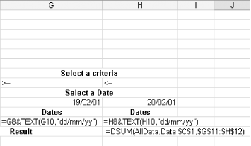
The end result should look like Figure, which, for the sake of demonstration, has all formulas displayed.
Figure. Worksheet showing correct formulas and headings

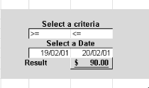
Hide rows 11 and 12, as you do not need to see them. You will end up with a simple-to-use table that looks like Figure below, which has had formatting applied for ease of reading.
Figure. Worksheet with final interface

By using this principle, you can easily have either one or a few database functions doing the work of what usually would require hundreds.