You might want to reference a single cell, such as cell A1, and then copy this reference across columns to the right. Naturally, this results in the formula reference changing to =B1, =C1, =D1, etc., which is not the result you want. You want the formula to increment by rows rather than columns-that is, =A1, =A2, =A3, etc.
Unfortunately, there is no option in Excel that lets you do this. However, you can get around this by using the INDIRECT function with the ADDRESS function nested inside.
Perhaps the best way to explain how to create the required function is to use an example with predictable results. In cells A1:A10, enter the numbers 1 through 10 in numerical order. Select cell D1, and in this cell enter the following:
=INDIRECT(ADDRESS(COLUMN( )-3,1))
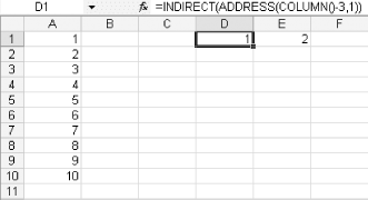
As soon as you enter this, the number 1 should appear in cell D1. This is because the formula references cell A1.
If you copy this formula across the column to the right, cell E1 will contain the number 2. In other words, although you are copying across columns, the formula reference is incrementing by rows, as shown in the figure.
This method is especially useful when a spreadsheet has headings going down rows in one column, and you want to create a dynamic reference to these row headings across other columns.

D1 to cell E1If you keep copying this to the right, cell F1 will contain the number 3, cell G1 will contain the number 4, etc. This is a fairly straightforward process if you are referencing only a single cell. Many times, however, you will need to reference a range of cells that is being used in the argument for a function.
We'll use the ever-popular SUM function to demonstrate what we mean. Assume you receive a long list of numbers, and your job is to sum the column of numbers in a running total fashion, like this:
=SUM($A$1:$A$2), =SUM($A$1:$A$3), =SUM($A$1:$A$4)
The problem occurs because the results need to be dynamic and to span across 100 columns on row 1 only, not down 100 rows in another column (as often would be the case).
Naturally, you could manually type such functions into each individual cell, but this would be very time-consuming. Instead, you can use the same principle as the one that you used when referencing a single cell.
Fill the range A1:A100 with the numbers 1 through 100 in numeric order. Enter 1 into cell A1, select cell A1, hold down the Ctrl key, left-click, and drag down 100 rows with the fill handle.
Select cell D1 and enter this formula:
=SUM(INDIRECT(ADDRESS(1,1)&":"&ADDRESS(COLUMN( )-2,1)))
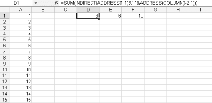
This will give you a result of 3, which is the sum of cells A1:A2. Copy this formula across to cell E1 and you will get a result of 6, which is the sum of cells A1:A3. Copy to cell F1 and you will get a result of 10, which is the sum of cells A1:A4.

D1 to cell F1The volatile COLUMN function caused the last cell reference to increment by 1 each time you copied it across to a new column. This is because the COLUMN function always returns the column number (not letter) of the cell that houses it unless you reference a different cell.
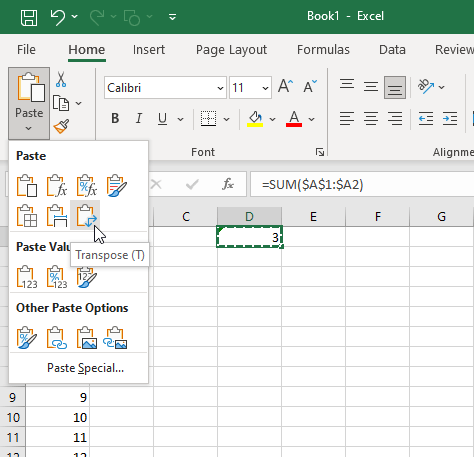
Use Paste Special » Transpose

Alternatively, you can use the Paste Special... » Transpose feature in Excel. Add the formula =SUM($A$1:$A2) to cell B1 (note the relative row absolute column reference to $A2), and then copy this formula down to cell B100. With B2:B100 selected, copy, select cell D1 (or any cell that has 100 or more columns to the right), and then select Transpose from the Home » Paste » Paste Special. If you like, you can delete the formulas in B2:B100.