When a range of cells contains one or more error values, most formulas that reference that range of cells also will return an error. You can overcome this frustration by using the DSUM function.
Assume you have a long list of numbers for which you need to get the sum total. However, one of the cells, for whatever reason, is returning the #N/A error.
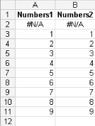
Set up some data such as that shown in the figure.
Figure. Data set up to generate #N/A error message

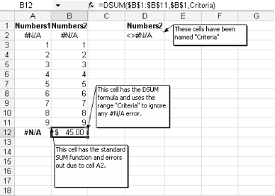
To generate the #N/A error, enter the formula =#N/A( ) in cells A2 and B2. Cell A12 uses a standard SUM function that sums cells A2:A11, and because cell A2 has the #N/A error, the SUM function also returns #N/A. The range D1:D2 has been named Criteria and is used as the last argument in the DSUM function, which resides in cell B12.
The syntax for the DSUM function (and all the database functions) is as follows:
=DSUM(database,field,criteria)
The database argument identifies the range of cells that comprise the list or database. Within the database range, rows of related information are treated as records, while columns of data are treated as fields. The first row contains labels for all the columns.
The field argument indicates which column is used in the function. The column can be identified by name using the labels at the top of the column, or it can be identified by position. The first column is 1, the fourth column is 4, and so on.
The criteria argument identifies a range of cells containing conditions. The range used for the criteria must include at least one column label plus at least one cell below the column label that specifies a condition for the column.
If the data you want to sum will likely contain a variety of different kinds of errors, you might need to consider using the DSUM function with a wide range of criteria to accommodate the possible errors. However, it is always best to address the error at the source and eliminate it whenever possible rather than work around it.
To work around it, you again use the DSUM function, but this time you need to set up criteria that span four columns, expanding the named range criteria to include D1:G2 via Insert » Name » Define, as shown in the figure.
Figure. The DSUM function used to ignore a number of different errors

Excel has a rich set of database functions, and you can use any one of them in the same way. Consider using the same method for DCOUNT, DCOUNTA, DMAX, DMIN, DPRODUCT, etc.