Sometimes you might need to use a single VLOOKUP formula to look in different tables of data set out in spreadsheets. One way in which you can do this is to nest several VLOOKUP functions together, telling them to look into a specified table depending on a number that you enter into another cell. For instance:
=IF(A1=1,VLOOKUP(B1,Table1,2,FALSE),IF(A1=2,VLOOKUP(B1,Table2,2,FALSE),""))
In this formula, you tell the VLOOKUP function to look in the named range Table1 if A1 contains the number 1 (IF(A1=1, VLOOKUP(B1,Table1,2,FALSE)), and to look in the named range Table2 if A1 contains the number 2 (IF(A1=2,VLOOKUP(B1,Table2,2,FALSE)).
As you can imagine, the formula will become very large and unwieldy if you use more than two nested IF functions. The following formula, for instance, uses only five nested functions, but it is very daunting!
=IF(A1=1,VLOOKUP(B1,Table1,2,FALSE),IF(A1=2,VLOOKUP(B1,Table2,2,FALSE),IF(A1=
3,VLOOKUP(B1,Table2,3,FALSE),IF(A1=4,VLOOKUP(B1,Table4,2,FALSE),IF
(A1=5,VLOOKUP(B1,Table5,2,FALSE),"")))))
Although the formula will return the desired results, you can make the formula a lot shorter, add more than five conditions, and end up with a formula that is very easy to manage.
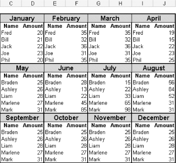
Assume you have 12 different tables set up on a spreadsheet, each representing a different month of the year. Each table is two columns wide and contains the names of five employees and five corresponding amounts. Each table has been named according to the month that it represents-i.e., January's data has a named range of January, February's data has a named range of February, and so on, as shown in the figure.
Figure. Twelve tables, each representing a month of the year

Select cell A1. Then select Data » Validation, and on the Settings tab select List from the Allow: box. In the Source: box, type each month of the year, separating each with a comma. It is vital that your named ranges for each table are the same as the month names you used in the validation list. Click OK.
Select cell B1 and set up a validation list as explained earlier, this time using the names of each employee. If the employee names are too large to type, simply reference a range of cells containing them for the source. Click OK.
In cell A2, enter this formula:
=VLOOKUP($B$1,INDIRECT($A$1),2,FALSE)
Select the required month from the list in cell A1 and the required employee name in the list in cell B1, and the formula in cell A2 will return the corresponding amount for that person for that month.
There are a few advantages to using this approach. If you are not familiar with the INDIRECT function, it is used to read the contents of a cell as a range address rather than as text. As you named 12 different ranges, each representing a month of the year, the formula using the INDIRECT function reads the word January as a range reference rather than as a text string.
Another advantage to using a formula with the INDIRECT function is that you can escape Excel's restriction of having only seven levels of nested functions.