To quickly insert subtotals in a list or table, you can use the Subtotal command on the Data tab. This will automatically create subtotal rows and group them for easy viewing. If you want to manually create the subtotals, you can use the SUBTOTAL function with a reference that changes based on the filter applied.
Subtotal Function
Although SUBTOTAL is one of Excel’s most convenient functions, you sometimes want to choose the function it uses, or apply it to data that can expand and contract.
You use the SUBTOTAL function in Excel to perform a specified function on a range of cells with AutoFilters applied to them. When the AutoFilter has been applied, the SUBTOTAL function will use only the visible cells; all hidden rows are ignored (but not manually-hidden rows). The operation it performs depends solely on the number (between 1–11 or 101–111 ) that you supply to its first argument, Function_num. For example:
=SUBTOTAL(1,A1:A100)
will average all visible cells in the range A1:A100 after AutoFilters have been applied. If all rows in A1:A100 are visible, it will simply average them all and give the same result as:
=AVERAGE(A1:A100)
The number for the first SUBTOTAL argument (Function_num), and its corresponding functions are shown in the following table:
| Function_Num Includes Manually Hidden Rows | Function_Num Ignores Manually Hidden Rows | Function Name |
|---|---|---|
| 1 | 101 | AVERAGE |
| 2 | 102 | COUNT |
| 3 | 103 | COUNTA |
| 4 | 104 | MAX |
| 5 | 105 | MIN |
| 6 | 106 | PRODUCT |
| 7 | 107 | STDEV |
| 8 | 108 | STDEVP |
| 9 | 109 | SUM |
| 10 | 110 | VAR |
| 11 | 111 | VARP |
Note: SUBTOTAL function will always ignore values in cells that are hidden using a filter. | ||
Because you need to use only a number between 1 and 11 (or 101 and 111), you can have one SUBTOTAL function perform whatever function you choose. You even can choose from a drop-down list that resides in any cell. Here is how to do this.
Make Subtotals Dynamic with a Drop-Down List
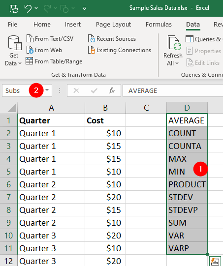
- Add all the function names, in the same order as in the above table, to a range of cells. For this example, we will use
D1:D11. - With this range selected, click the Name box (the white box on the left of the Formula bar) and type the name
Subs. Then click Enter.
- Hide the
Dcolumn. Select columnDin its entirety and then right-click on it and chooseHidefrom the context menu. - Go to the
Developertab and clickInsertfrom theControlsgroup, choose theCombo Boxicon under the Form Controls section. - Click cell
C2, to have your Combo Box automatically snap to the size of the column and row it resides in, hold down yourAltkey at the same time as you size the Combo Box.
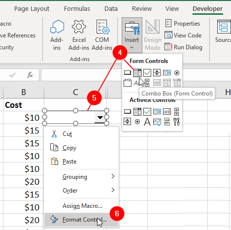
- Right-click the Combo Box and choose
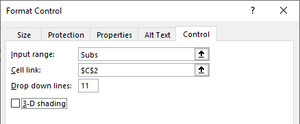
Format Control. - The Format Control dialog box will displayed. Choose the
Controltab and follow these instructions:- In the
Input range, typeSubs. - In the
Cell Linkbox, type$C$2. - In the
Drop down lines, type 11.
- In the
- In cell
C3, enter this formula:
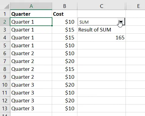
=IF($C$2="","","Result of "&INDEX(Subs,$C$2))
In cell C4, enter this formula:
=IF($C$2="","",SUBTOTAL($C$2,$B$2:$B$13))
where $B$2:$B$13 is the range on which the SUBTOTAL should act.
Now all you need to do is select the required SUBTOTAL function from the Combo Box and the correct result will be displayed, as shown in the figure.