Filter a Data Range
Using filters you can easily analyze and view specific subsets of your data based on different conditions or criteria. To apply filter, follow these steps:
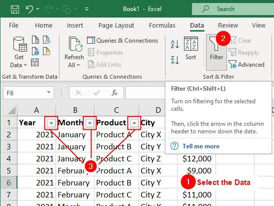
- Select the range of cells that you want to filter. This can be a single column or multiple columns with headers.
- Go to the
Datatab, in theSort & Filtergroup, click on theFilterbutton or pressCtrl+Shift+Lto toggle the filter on/off. - Excel will add filter dropdown arrows to the headers of the selected columns. See following figure:
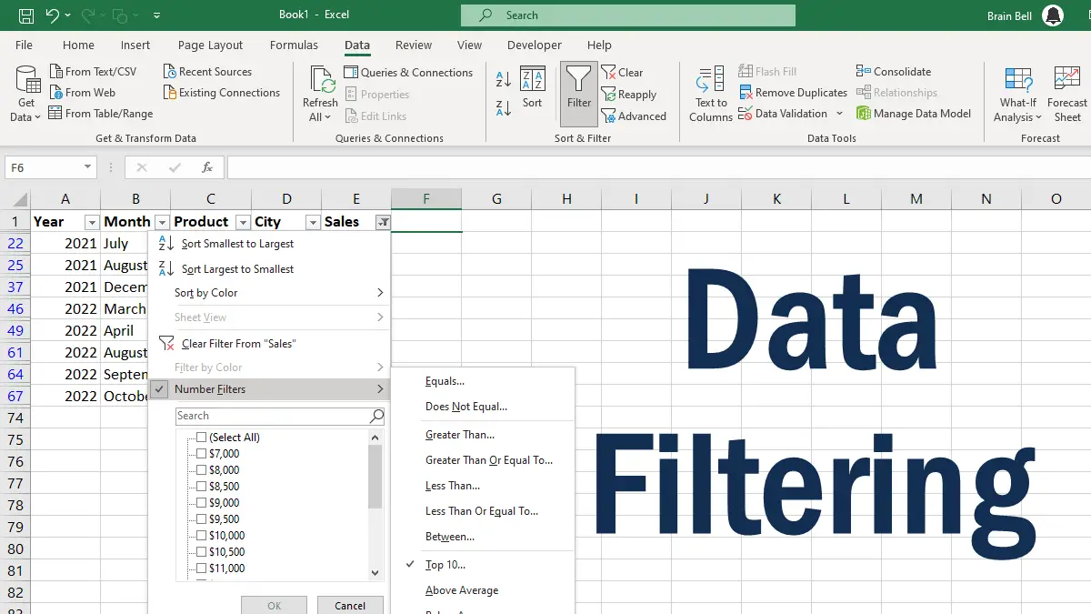
- Click on the filter arrow in the column header you want to filter. A dropdown list will appear with unique data entries in the column and additional searching, sorting, and filtering options (such as text filters, number filters, date filters, etc. depending on the column data).
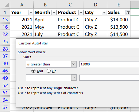
- Choose the filter criteria that you want to apply. For example, if you’re going to filter a column for values greater than a certain number, you can select
Number Filters > Greater Thanand enter the desired value in the Custom AutoFilter dialog box.
Excel will filter the data based on your selection, hiding the rows that do not meet the specified criteria as shown in the following figure:
You can apply filters to multiple columns by selecting the desired filter criteria for each column separately.
To remove the filters and show all the data again, go back to the Data tab and click on the Filter button again or use the keyboard shortcut Ctrl+Shift+L.
Filter Data For The Top Items
Suppose you want to see the top ten items based on the Sales. You can use the (Top 10…) AutoFilter option to filter a range by the largest number or smallest number. To filter and display only the top 10 items follow this step-by-step guide:
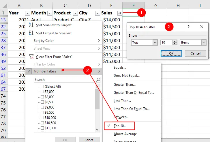
- Click on the filter drop-down arrow in the
Salescolumn header. This will open a list of options for that column. - In the filter options, select
Number Filters >Top 10option. - The Top 10 AutoFilter box will appear, allowing you to choose how many items you want to display. By default, it’s set to show the top 10 items. If that’s what you want, simply click
OK.
Excel will now show only the top 10 items in the filtered data. The rest of the data will be hidden from view.
Clear Filter
If you make changes to the data or want to remove the filter later, you can simply click on the filter drop-down arrow again and choose Clear Filter from [Column Name].