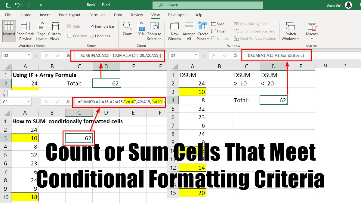
How can I calculate only the cells with a specific background color?
- SUMIF Function
- SUMIFS Function
- DSUM Function
- Alternatives to SUMIF and SUMIFS Function for Earlier Excel Versions.
Use SUMIF Function
You can use the SUMIF function to add a range of cells that meet a particular criterion (only one criterion). If you need to deal with more than one factor, you can use SUMIFS function (or an array formula for earlier Excel versions).
For example, you have a list of numbers in the range A2:A15. You applied conditional formatting to these cells so that any numbers less than the value 20 are highlighted, as shown in the figure:
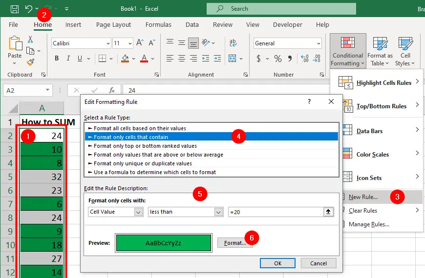
Now you need to sum the value of the highlighted cells that meet the conditional formatting criteria. The SUMIF function is a useful tool for adding up values that meet a certain condition. The syntax of the SUMIF function is:
=SUMIF(range, criteria, [sum_range])
range– the range of cells that you want to apply the criteria to.criteria– the condition that defines which cells will be summed.sum_range– (optional) the range of cells that you want to sum. If you omit this argument, the function will sum the cells in therange(first) argument.
To sum cells containing values less than 20, we can use this formula:
=SUMIF(A2:A15, "<20")
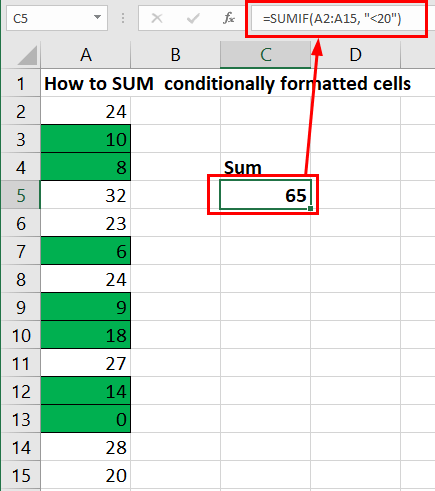
This formula will check each cell in the range and see if it meets the criteria. If it does, it will add it to the sum. If not, it will ignore it.
Use SUMIFS Function
For example, you have a long list of numbers in the range A2:A100. You applied conditional formatting to these cells so that any numbers that fall between the range of 10 and 20 are flagged.
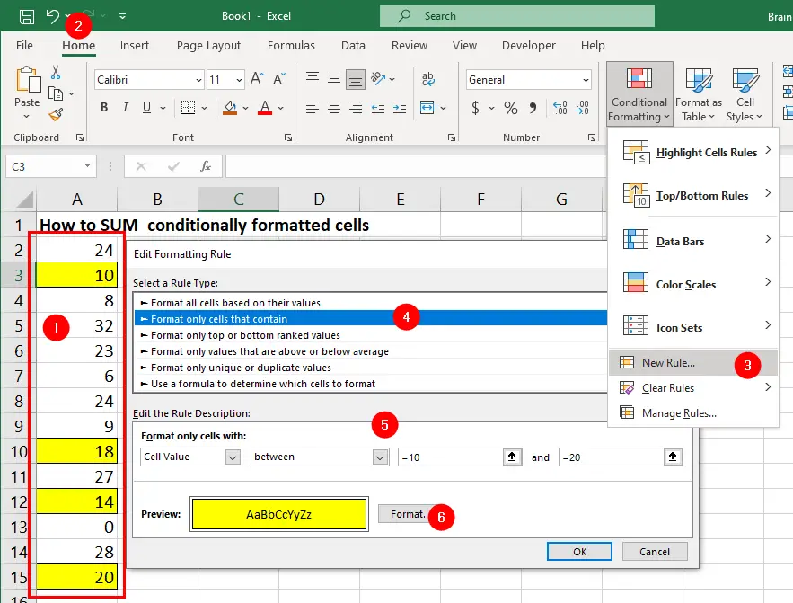
Now you have to add the value of the cells that meet the criterion you just set and then specify the sum of the values using conditional formatting.
You don’t need to worry about what conditional formatting you applied to these cells, but you do need to know the criteria that were used to flag the cells (in this case, cells with values between 10 and 20).
The SUMIFS function in Excel allows you to add up the values in a range of cells that meet multiple criteria. The syntax of the SUMIFS function is:
=SUMIFS(sum_range, criteria_range1, criteria1, [criteria_range2, criteria2], ...)
sum_range– the range of cells that you want to sum up.criteria_range– the ranges of cells that you want to apply thecriteriato.criteriathe conditions that you want to match withcriteria_range.[criteria_range2, criteria2],...– You can define up to 127 pairs of criteria_range and criteria arguments.
To sum cells containing values between 10 and 20, we can use this formula:
=SUMIFS(A2:A15,A2:A15, ">=10", A2:A15, "<=20")
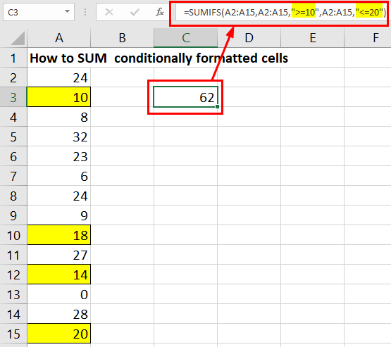
This formula will return 62, which is the sum of the values between 10 and 20 in the provided range.
Using DSUM Function
The preceding methods certainly get the job done, but Excel provides yet another function that enables you to specify two or more criteria. This function is part of Excel’s database functions, and is called DSUM.
To test it, use the same set of numbers in A2:A100 and follow these steps:
- Select cells
C1:D2 - Name this range
SumCriteriaby selecting the cells and entering the name in the name box to the left of the Formula bar. - Select cell
C1and enter=$A$1, a reference to the first cell on the worksheet. - Copy this across to cell
D1, and you should have a double copy of your column A heading. These copies will be used as headings for yourDSUMcriteria (C1:D2), which you calledSumCriteria. - In cell
C2, enter>=10. In cellD2, enter<=20. - In the cell where you want your result, enter the following code:
=DSUM($A$1:$A$100,$A$1,SumCriteria)
DSUM is the preferred and most efficient method of working with cells that meet certain criteria.
Array Formula as an Alternative for SUMIF and SUMIFS
You use an array formula like this:
=SUM(IF(A2:A100>=10, IF(A2:A100<=20, A2:A100)))

For earlier versions of Excel (97-2003), when entering array formulas, don’t press Enter. Press Ctrl+Shift+Enter. This way, Excel will place curly brackets around the outside of the formula so that it looks like this:
{=SUM(IF(A2:A100>=10,IF(A2:A100<=20,A2:A100)))}
If you enter these brackets yourself, it won’t work. You must allow Excel to do it for you.
Also, note that using an array formula can slow down Excel’s recalculations if there are too many references to large ranges.
Conditional Formatting
- Setting Up Checkboxes for Conditional Formatting
- Highlighting Formula Cells with Conditional Formatting
- Sum Cells That Meet Conditional Formatting Criteria
- Highlight Every Other Row or Column with MOD Function and Conditional Formatting
- Enable and Disable Conditional Formatting with a Checkbox
- Sort Data By Conditional Formatting Criteria
