- Sort Data Based on Cell Color
- Sort Data Based on Font Color
- Sort Data Based on Conditional Formatting Icon
Sort Data Based on Cell Color
To sort data based on cell color in Excel, you can follow these steps:
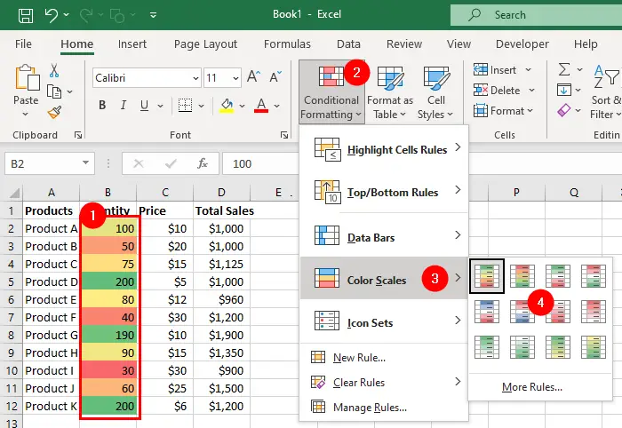
- Select the data that you want to apply conditional formatting. We selected
B2:B12. - Go to the
Hometab and click onConditional Formattingin theStylesgroup. - Choose
Highlight Cells RulesorColor Scalesoption. - Choose the colors that will determine how the cells are formatted.
This will apply the conditional format to the range. Next, follow these steps to sort the data based on cell colors (that we applied with the conditional formatting):
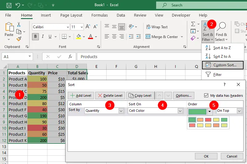
- Select the data/range.
- Go to the
Hometab and click onSort & Filterin theEditinggroup. - In the Sort dialog box, choose the column that you applied the conditional formatting from the
Sort bydrop-down list. - Under
Sort on, chooseCell Colorfrom the drop-down list. - Under
Order, choose the color that you want to stay on the top or bottom. - Click OK to close the Sort dialog box.
Sort Data Based on Font Color
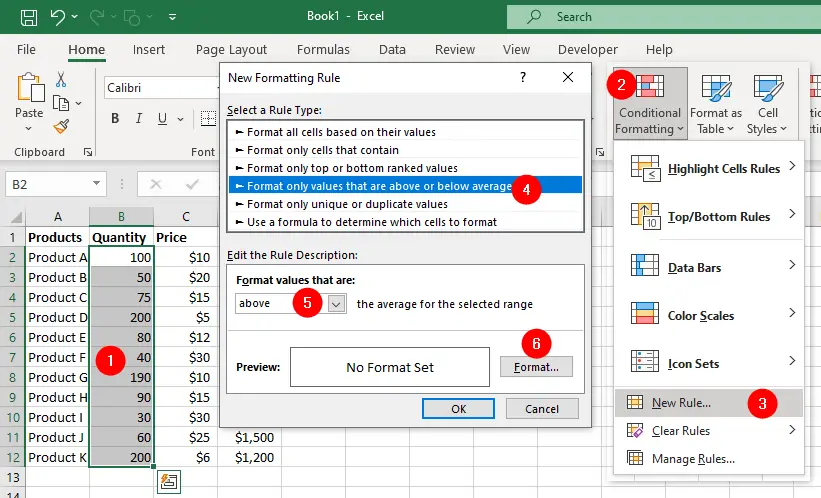
- Select the data that you want to apply conditional formatting. We selected
B2:B12. - Go to the
Hometab and click onConditional Formattingin theStylesgroup. - Choose
New Rule, it opens the New Formatting Rule dialog box. - Choose Format only values that are above or below average.
- Choose
abovefrom the Format values that are: menu. - Click
Formatbutton, it opens the Format Cell dialog box.
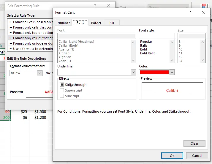
- Select
Fonttab in the Format Cell dialog box and choose a color (Green) from theColormenu. - Click OK twice to return back to the sheet.
- Now repeat all the above steps again and in step 5 choose
belowand choose a different font color for lower values.
The above steps apply the conditional formatting (green color) on cells that hold values above the average of selected cells and red color on cells that contain values lower than the average of selected cells.
Now follow these steps to sort the data based on font color (that we applied with the conditional formatting):
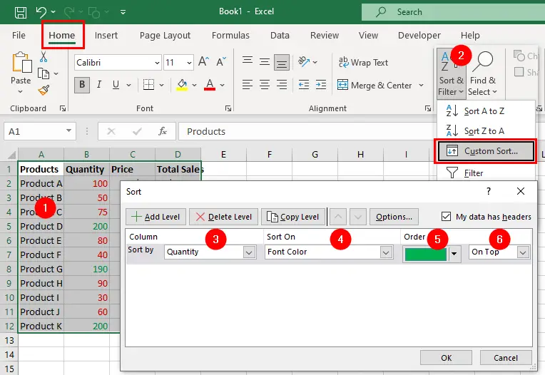
- Select the range of cells or the table you want to sort.
- Click on the
Sort & Filterbutton in theHometab and chooseCustom Sort. - In the
Sortdialog box, choose the column that contains the font color you want to sort by from theSort bydropdown list. - In the
Sort Ondropdown list, selectFont Color. - Choose the desired color in the
Orderdropdown list. - Specify the sort order, either
On ToporOn Bottom. - Click the OK button to apply the sorting.
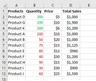
Excel will rearrange the data based on the selected font color. The rows with the specified color will be sorted according to the chosen sort order.
Sort Data Based on Conditional Formatting Icon
To sort data based on conditional formatting icons in Excel, you can follow these steps:
- Select the data that you want to apply conditional formatting. We selected
B2:B12. - Go to the
Hometab and click onConditional Formattingin theStylesgroup. - Choose
Icon Setsoption. - Choose the icon that will determine how the cells are formatted.
Next, in the Sort dialog box choose the column that contains the conditional formatting icons you want to sort by from the Sort On dropdown list, you can follow these steps:
- Select the range of cells or the table you want to sort.
- Click on the
Sort & Filterbutton in theHometab and chooseCustom Sort. - In the
Sortdialog box, choose the column that contains the font color you want to sort by from theSort bydropdown list. - In the
Sort Ondropdown list, selectConditional Formatting Icon. - Choose the desired icon in the
Orderdropdown list. - Specify the sort order, either
On ToporOn Bottom. - Click the OK button to apply the sorting.
Excel will rearrange the data based on the selected conditional formatting icon. The data or table with the specified icon will be sorted according to the chosen sort order.
Conditional Formatting
- Setting Up Checkboxes for Conditional Formatting
- Highlighting Formula Cells with Conditional Formatting
- Sum Cells That Meet Conditional Formatting Criteria
- Highlight Every Other Row or Column with MOD Function and Conditional Formatting
- Enable and Disable Conditional Formatting with a Checkbox
- Sort Data By Conditional Formatting Criteria