This tutorial covers Excel versions 365, 2007, and above, for older versions (i.e. 97-2003) visit the Conditional formatting and checkboxes in Excel 2003.
The checkboxes return either a TRUE or FALSE value (checked/not checked) to their linked cell. By combining a checkbox with conditional formatting, you can turn conditional formatting on and off via a checkbox.
Enabling Developer Tab
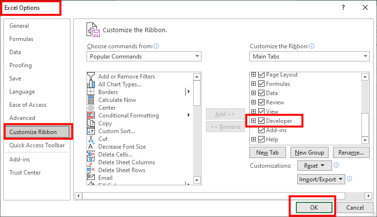
The first step is to insert checkboxes in your worksheet. If the Developer tab is not visible, enable it from the Excel Options > Customize Ribbon by checking the Developer option:
Inserting the checkboxes:
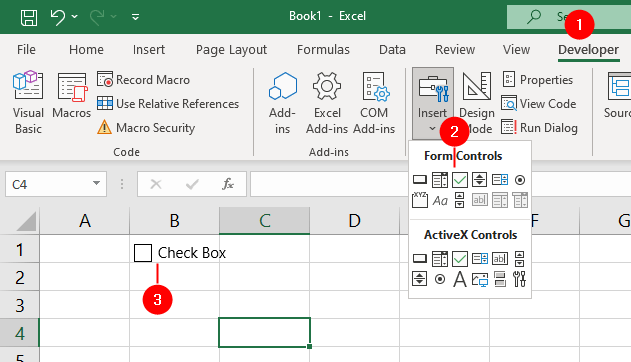
- Go to the
Developertab and click onInsertin the Controls group. - Select the
Checkboxoption from the Form Controls section. - Click anywhere on the worksheet to draw a checkbox.
- Edit the text next to the checkbox by clicking on it and typing your desired label.
The next step is to link each checkbox to a cell that will store its value. To do this:
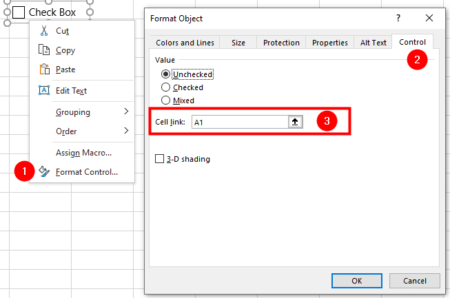
- Right-click on the checkbox and select
Format Control. - Go to the
Controltab and click on theCell linkbox. - Enter a cell reference or select a cell from your worksheet.
- Click OK.
The cell will display TRUE if the checkbox is checked, and FALSE if it is unchecked.
Set up conditional formatting:
The final step is to apply conditional formatting based on the checkbox values:
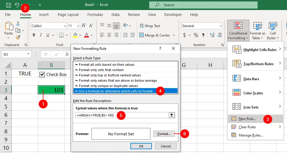
- Select the cells that you want to format with the checkbox.
- Go to the
Hometab and click onConditional Formattingfrom the Styles group. - Select
New Rule. - Choose
Use a formula to determine which cells to formatfrom the “Select a Rule Type” section. - You can then enter a formula that references the cell linked to the checkbox.
For example, if you want to format a cell B3 containing a value greater than 100 while the checkbox in A1 is checked, you can enter =AND(A1=TRUE,B3>100) as the formula.
- Click on
Format. - Choose your desired formatting options from the Font, Border, and Fill tabs.
- Click OK to confirm your rule and apply it to your selected cells.
The conditional formatting will be applied to the B3 if its value is greater than 100 and the checkbox is checked.
Conditional Formatting
- Setting Up Checkboxes for Conditional Formatting
- Highlighting Formula Cells with Conditional Formatting
- Sum Cells That Meet Conditional Formatting Criteria
- Highlight Every Other Row or Column with MOD Function and Conditional Formatting
- Enable and Disable Conditional Formatting with a Checkbox
- Sort Data By Conditional Formatting Criteria