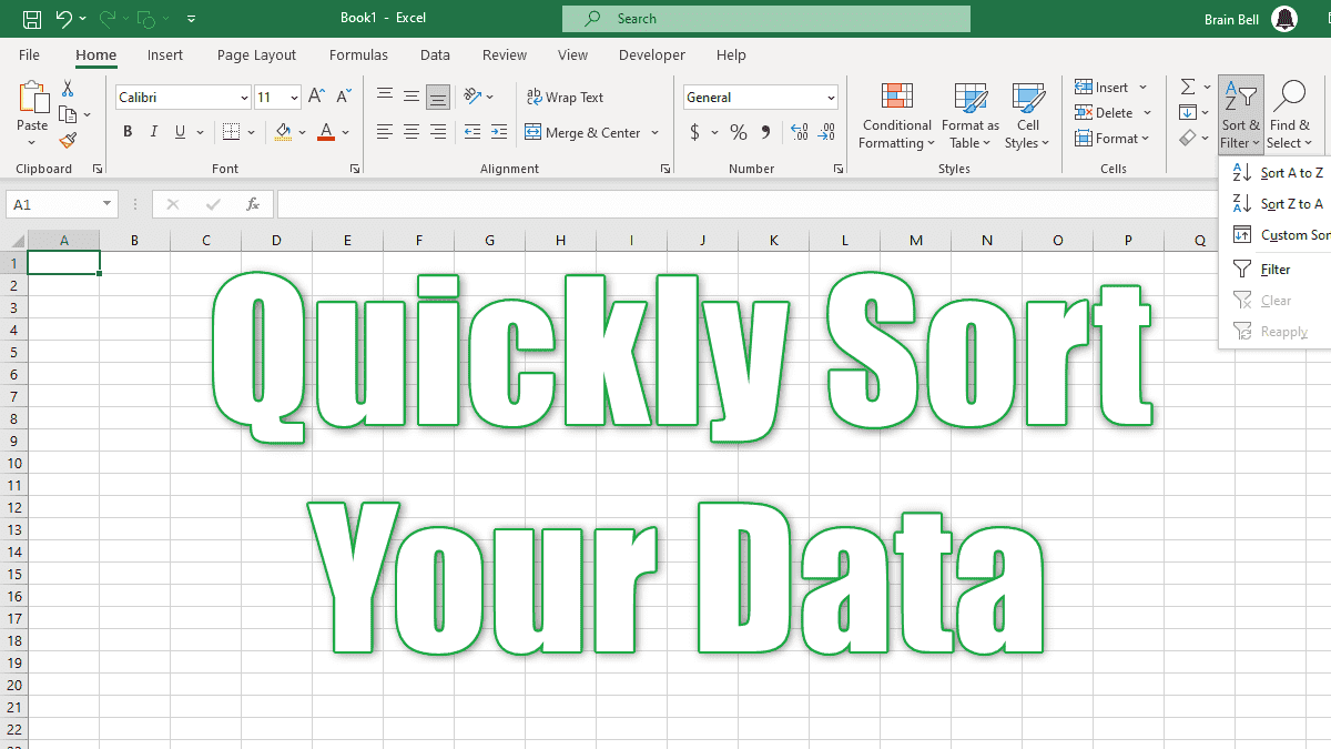
You normally sort the records or rows of a table by the values in one or more columns of the list or table. However, Excel also lets you sort by the font color, fill color, or cell icons that you apply to them with conditional formatting criteria. This is how you can do it.
Author: BrainBell
Quickly Sort Your Data
You can quickly rearrange or sort the records in a data range based on the data in a single column by first activating a cell in the column and then clicking the A-Z or Z-A option in the Sort & Filter group on the Data tab.
Cell Comments
Comments in Excel are small notes or annotations that you can add to a cell to provide additional information or context. Comments are useful for documenting your work, explaining formulas or functions, or giving feedback to others.
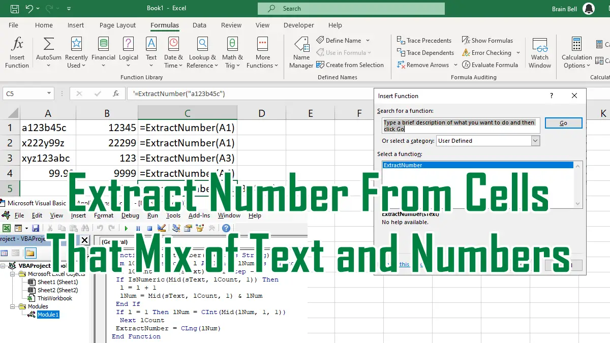
Sometimes you need to extract the numeric portion from a cell that contains both text and numbers. For example, if you have a cell that contains “Product ID: 12345”, you may want to get only the number “12345”. There are different ways to do this, we will demonstrate some methods and examples for doing this task.
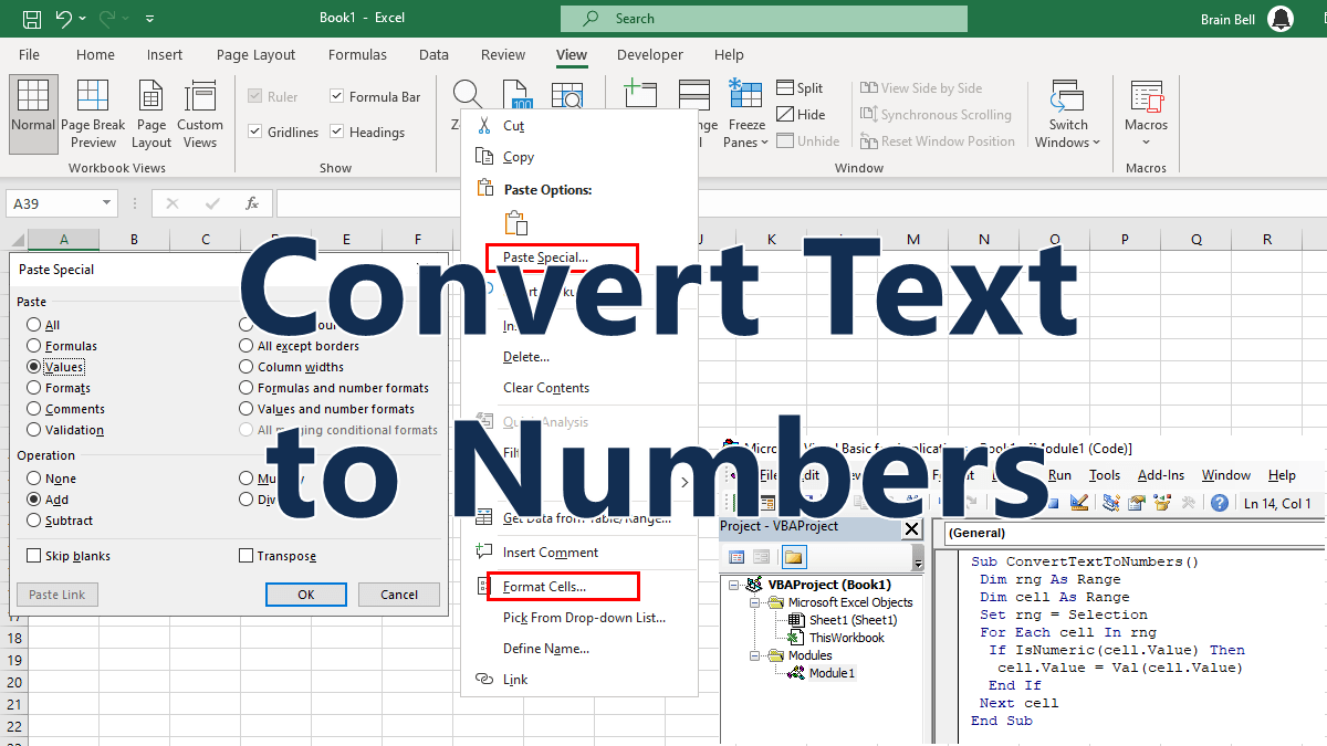
Convert Text to Numbers
The contents of a cell might look like numbers, especially in imported data, but it still might be impossible to use these numbers in calculations. Here are a few ways in which you easily can convert these “text” numbers to true numbers.
Using Code and Char Functions
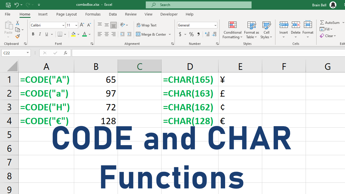
The CHAR and CODE functions in Excel are useful for working with characters and their numeric codes. The CHAR function returns the character corresponding to a given numeric code, while the CODE function returns the numeric code of a given character.
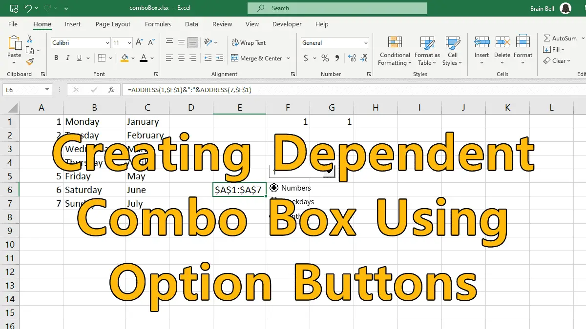
Accessing three lists of choices simultaneously generally requires that you use three separate controls, such as three ComboBox control. Instead, you can use a ComboBox in combination with option buttons (also called radio buttons) to have a list change automatically according to which option button you choose.
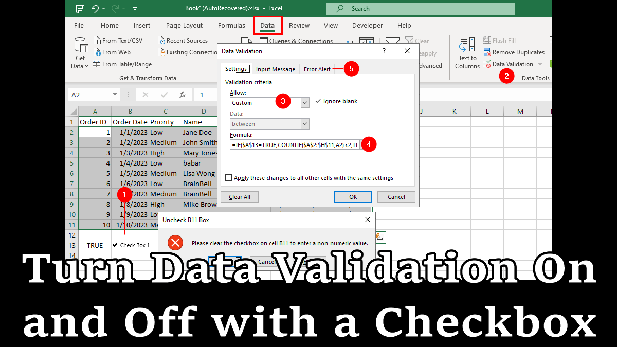
One way to prevent users from entering wrong data is to use data validation. Data validation limits the type of data that can be entered in the cells. Sometimes, you might want to allow users to enter data that is not allowed by the data validation rules. Instead of removing the data validation, you can use a simple checkbox to override it.
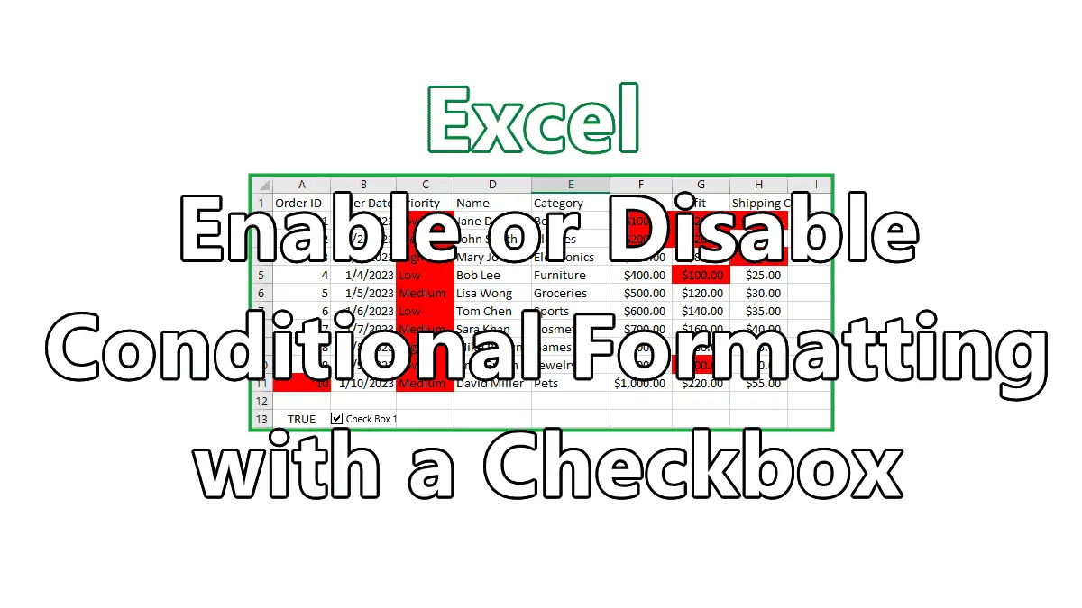
Conditional formatting is a powerful feature of Excel that lets you change the appearance of cells based on their values. However, using the menus and dialog boxes of the GUI to apply and remove conditional formatting can be tedious and time-consuming. A better way to control conditional formatting is to use checkboxes on your worksheet that let you switch it on and off easily and quickly. This way, you can view your data in different ways whenever you want, without going through multiple steps.
Create 3D Effects in Tables or Cells
Whenever you see a nifty 3D effect in a program or application such as Excel, you are actually seeing an illusion created by specific formatting. It is easy to create this illusion yourself by applying formatting to a cell or range of cells.