Named Value
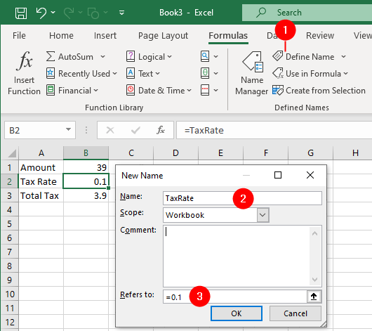
Assume you have a tax rate of 10%, which you need to use throughout your workbook for various calculations. Instead of entering the value 10% (0.1) into each formula that requires this tax rate, you can enter the word TaxRate and Excel automatically will know that TaxRate has a value of 0.1. Here is how to do this:

- Click on the
Formulastab and in the “Defined Names” group, click onDefine Name. - In the Name box, type
TaxRate. - In the Refers To box, enter
=0.1 - Click OK.
From this point on, you can enter any formula into any cell, and instead of adding 10% as part of the calculation, you can use the word TaxRate.
Define Name to Sum Cells Automatically
To take things a step further with this concept, you can use formulas as your Refers To range rather than a cell address or constant value. Suppose you want to create a name that, when entered into a cell, automatically returns the SUM of the 10 cells immediately above it.
- Select cell
A11on any worksheet. - Click on the
Formulastab and in the “Defined Names” group, click onDefine Name. - In the Name box, type
Total. - In the Refers To box, enter
=SUM(A1:A10). - Click OK.
Enter any 10 numbers in any column starting from row 1. Now come down to row 11 of the same column and type the following: =Total.
The name Total automatically will return the SUM of the 10 cells you just entered in A1:A10.
If you want to create a similarly named formula that is not restricted to only 10 cells, but rather, includes all the cells directly above whatever row happens to contain =Total, follow these steps.
- Select cell
B11and then - Click on the
Formulastab and in the “Defined Names” group, click onDefine Name. - In the Name box, type
Total2. - click the Refers To box and type the formula
=SUM(B$1:B10). - Click OK.
Select any row in any column other than row 1 and enter =Total, and you automatically will get the SUM of all the cells above where you enter this, regardless of how many rows there are.
This is because you anchored row number 1 by making it an absolute reference, yet left the reference to cell B10 as a relative reference, meaning it always will end up being the cell immediately above where you entered the named formula =Total.
Generate Names From the Selection
Excel can generate named ranges based on your selection, using the top/bottom rows and/or left/right columns as the names. These named ranges can then be used to reference the data. To generate names from the selection follow these steps:
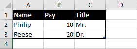
- In cell
A1, enter the headingName. - In cell
B1, enter the headingPay. - In cell
C1, enter the headingTitle. - In cell
A2, enterPhilip. - In cell
A3, enterReese. - In cell
B2, enter10. - In cell
B3, enter20. - In cell
C2, enterMr. - In cell
C3, enterDr.

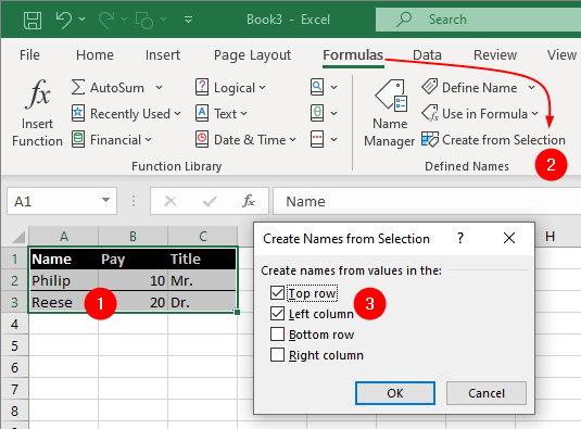
- Now, select the range
A1:C3. - Go to the
Formulatab and clickCreate from Selection. It will open the “Create Names from Selection” dialog box. - Ensure that both the Top row and Left column checkboxes are checked.
- Click
OK.

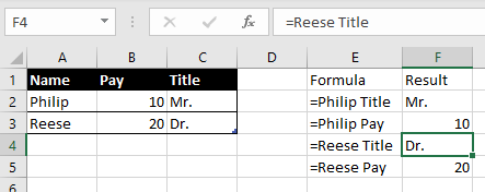
Select any cell outside your table and enter =Reese Title. You should get the correct title (in this case Dr. ) for the name Reese. See the following figure:

The space between the words Reese and Title is important, as this is what Excel understands as the intersect operator.
Note: The names of named ranges cannot contain a space. When you create names from a selection, Excel automatically places an underscore in the spaces between two or more words. To refer name that contains spaces, you should replace the spaces with underscores. For example, to refer Carl Nicks, you should use Carl_Nicks.