Cell References

Most formulas we create include references to cells, range (a collection of cells), or the name. These references enable formulas to work dynamically with the values contained in those cells.

For example, if a formula refers to cell C6 and you change the value contained in C6, the formula result changes to reflect the new value. If you didn’t use references in your formulas, you would need to edit the formulas themselves to change the values used in the formulas. We can divide cell references into four types:

1. Relative Reference
2. Absolute Reference
3. Mixed Reference
4. Named Reference

We’ll also discuss the following topics:

• Name Manager
• Move relative references without making the reference absolute

Relative Reference

A relative reference is a cell address that changes when the formula is copied to another location. By default, Excel uses relative references in formulas.

For example, if you have a formula =A1*C1 in cell E1, and you copy it to cell E2, the formula will change to =A2*C2.

This is because the formula refers to the cells that are in the same position relative to the formula cell. Relative references are useful when you want to apply the same calculation to different cells.

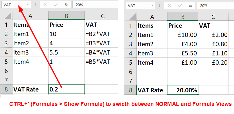
Press Ctrl+` (or go to Formula tab and click Show Formula in Formula Auditing group) to see the formula in each cell instead of the resulting value:

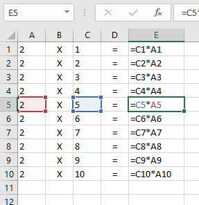
The formulas for E2 to E10 are created by copying and pasting E1. The cell references in the formula are relative to the position of the cell containing them and are automatically updated for the new location.

You can recognize a relative reference by the absence of the $ sign before the column and row coordinates, such as A1 or B1:D10.

Absolute Reference

When you refer to a cell in a formula using the absolute reference format, Excel uses the physical address of the cell, and the row & column references don’t change when you copy or fill the formula to other cells.

An absolute reference uses two dollar signs $ in its address: one for the column letter and one for the row number, for example, $A$1.

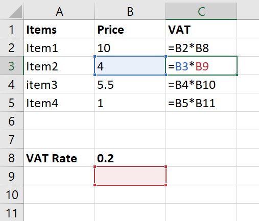
In the following example, we need to calculate the VAT for each item separately. The value of cell C2 for the Item1 would be =B2*B8. If you create formulas for C3, C4 and C5 by copying and pasting C2, you’ll receive the incorrect result because reference to the relative reference B8 would be incremented to B9, B10 and then B11:

To fix the error we need to fix the reference to B8, so that it doesn’t change when the formula is copied. Let’s edit the formula in C2 cell and place a $ symbol in front of the row and column addresses i.e. $B$8: Now copy C2 cell (containing formula) and paste it on C3, C4 and EC5, you’ll see the reference $B$8 doesn’t change, so the results are correct:

Shortcut Key to Convert Relative Reference into Absolute:
When entering a formula, press F4 (or ⌘+T) to convert the B8 to $B$8.

The $ signs tell Excel that B8 is an absolute reference. When you copy and paste this formula from C2 to C3, the formula will change as follows: =$B$8*B3.

Because we copied the formula to the cell in the next row down, B2 has changed to B3. But the reference to B8 hasn’t changed because you identified it as an absolute reference.

Absolute references are helpful when you need to use a constant value in your calculations, or when you want to preserve the original references of a formula when copying it to other cells.

Mixed Reference

We already learn that relative reference changes when a formula is copied to another cell, while an absolute reference remains constant.

A mixed cell reference in Excel is a type of cell reference that combines relative and absolute references. A mixed cell reference has either an absolute column and a relative row, or an absolute row and a relative column.

• $A1 is a mixed-cell reference with an absolute column and a relative row. The column A will not change, but the row will adjust relative to the new location of the formula.
• A$1 is a mixed cell reference with a relative column and an absolute row. The row 1 will not change, but the column will adjust.

Mixed cell references are useful when you want to fix one part of a cell reference in a formula, but allow the other part to change dynamically.

Named References

Names create absolute references to cells or range in the current worksheet. They can be used in formulas, and when these are copied (or dragged by the fill handle), the references will not be incremented or changed. To create a name for a cell or cell range:

1. Select the cell (B8 in our example) you want to name
2. Click the Name box (showing B8), on the left of the Formula Bar
3. Type the name that you’ll be using to refer to the selection, then press Enter

You can change an absolute reference into Named references by naming the cell or range and then use the name in the formula. In our Absolute reference example, we used the $B$8 cell reference for VAT value, now we’ll change the name of B8 cell into VAT and convert our formula =B2*$B$8 to =B2*VAT:

Name Manager

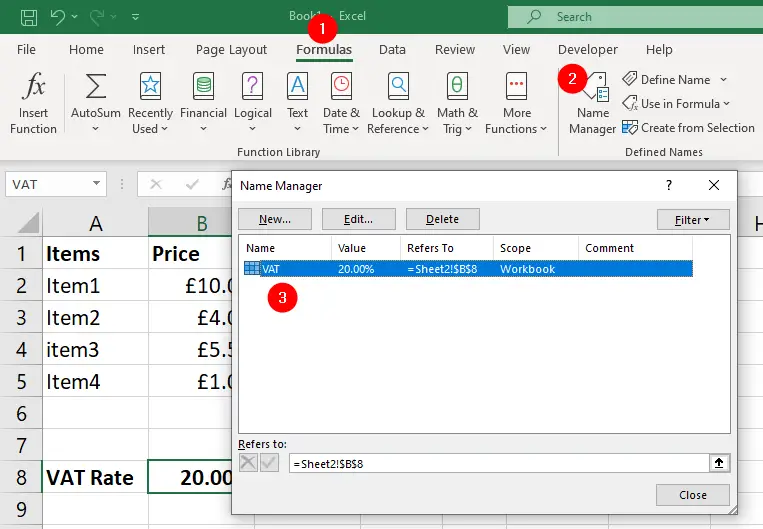
To view the list of Named References in the workbook, click the Formulas tab and select the Name Manager:

Move relative references without making the reference absolute

In Excel, a formula reference can be either relative or absolute, but sometimes you want to move cells that use relative references without making the references absolute. Here’s how.

If you already set up your formulas using only relative references, or perhaps a mix of relative and absolute references, you can reproduce the same formulas in either another range on the same worksheet, another sheet in the same workbook, or perhaps even another sheet in another workbook.

To do this without changing any range references inside the formulas:

1. Select the range of cells you want to copy
2. Select Home » Find & Select » Replace.
3. In the Find What: box, type an equals sign (=)
4. In the Replace With: box, type an at sign (@).
5. Click Replace All.
6. The equals sign = in all the formulas on your worksheet will be replaced with the at @ sign.

You now can simply copy this range, paste it to its desired destination, and follow these steps:

1. Select the range of cells you’ve just pasted
2. Select Home » Find & Select » Replace.
3. In the Find What: box, type an at sign (@)
4. In the Replace With: box, type an equals sign (=).
5. Click Replace All.
6. The at @ sign in all the formulas on your new location will be replaced with the = equal sign.

Your formulas now should be referencing the same cell references as your originals.

---

Understanding Workbooks and Worksheets: