- Same Name to a Range on Multiple Worksheets
- Relative Reference Named Range
- Use a Function in a Named Range
Same Name to a Range on Multiple Worksheets
Assume you have a workbook with three worksheets. These three worksheets are simply named Sheet1, Sheet2, and Sheet3. You want to have a named range called MyRange that will refer to the range Sheet1 A1:A10 when on Sheet1, Sheet2 A1:A10 when on Sheet2, and Sheet3 A1:A10 when on Sheet3.
To do this, activate Sheet1, select the range A1:A10, and then click in the Name box, as you did in Address Data By Name. Type Sheet1!MyRange and then press Enter. Do the same for Sheet2 and Sheet3, typing Sheet2!MyRange and Sheet3!MyRange, respectively.
Now activate any sheet and click the drop arrow on the Name box. You should see only one occurrence of the name MyRange. Select this and you will be taken directly to the range A1:A10. Now activate any other sheet and do the same. You always will be taken to the range A1:A10 of that sheet.
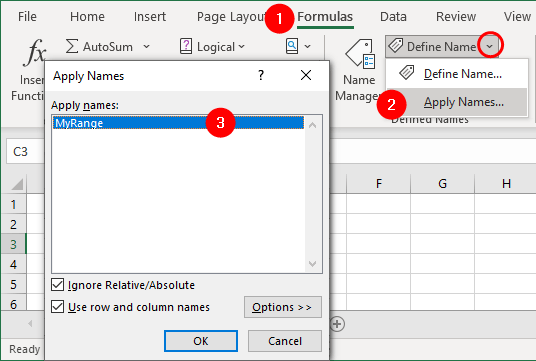
You can do this because you preceded the name with the sheet name followed by ! (an exclamation mark). If you go to the Formula » Define Name » Apply Names, you will see only one name: the one that refers to the currently active sheet. See the following figure:
Referring a worksheet name if it includes spaces:
If your worksheet name includes spaces, you cannot simply refer to the range Sheet1 A1:A10 as Sheet1!MyRange. Instead, you must call it 'Sheet 1'!MyRange, putting a single apostrophe around the word Sheet1. In fact, you also can use single apostrophes with a worksheet name with no spaces, so it is a good idea always to use single apostrophes when referring to worksheet names to cover all your bases.
Relative Reference Named Range
You can use a relative reference named range as well. By default, named ranges are absolute, but you do not have to leave them this way. Try the following:
- Select cell
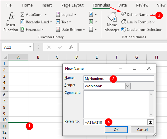
A11on any worksheet and then - Select
Formula » Define Nameto open the New Name dialog box. - In the Name box, type
MyNumbers. - In the Refers To box, type
=A$1:A$10and then - Click OK.
Now enter the number 1 in cell A1, Select cell A1, move your cursor to the fill handle, and press the left mouse button. While holding down the Ctrl key, drag down to cell A10.
Holding down the Ctrl key with a single number will cause Excel to create a list incremented by 1.
Enter 1 in cell B1 and drag down to cell B10, without holding down the Ctrl key this time.
- Into cell
A11, enter the following formula:=SUM(MyNumbers) - In cell
B11, enter this formula:=SUM(MyNumbers)
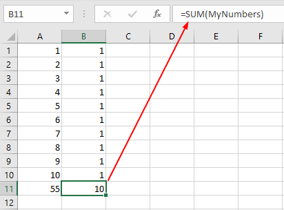
You should get 55 and 10, respectively, because cell A11 was active when you defined the new name and referred the range name to A$1:A$10, which is a relative column and absolute row named range.
The dollar sign ($) forces any range to be absolute.
When you use the name MyNumbers in a formula, it always will refer to the 10 cells immediately above the formula. If you use =SUM(MyNumbers) in cell A11 of another worksheet, it still will refer to cells A1:A10 on the sheet that was active when you originally created the range name.
Use a Function in a Named Range
Suppose you want to simplify the summing of the 10 cells mentioned earlier:
- Select cell
A11on any worksheet and then - Select
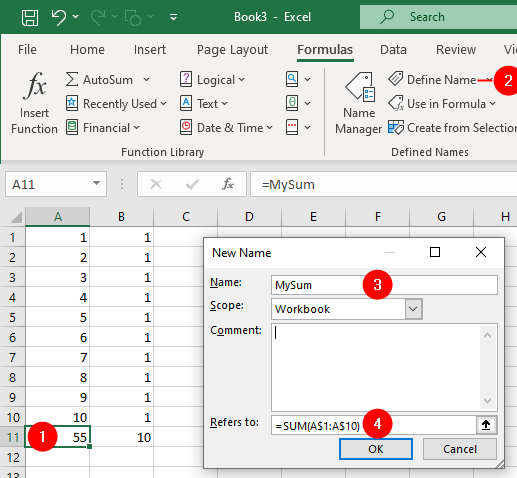
Formula » Define Nameto open the New Name dialog box. - In the Name box, type
MySum. - In the Refers To box, type
=SUM(A$1:A$10)and then - Click OK.
Now enter the number 1 in cell A1, Select cell A1, move your cursor to the fill handle, and press the left mouse button. While holding down the Ctrl key, drag down to cell A10.
Enter 1 in cell B1 and drag down to cell B10, without holding down the Ctrl key this time.
- In cell
A11, enter the following formula:=MySum - In cell
B11, enter this formula:=MySum
You will get the same results you got before, but without requiring the SUM function. Mixing up the absolute and relative references and nesting a few functions together can be very handy and can save a lot of work.