One of the best things about using conditional formatting is that your spreadsheet’s formula identification capabilities will be dynamic. This means that if you add or remove a formula, your formatting will change accordingly. Here we explain how to do this.

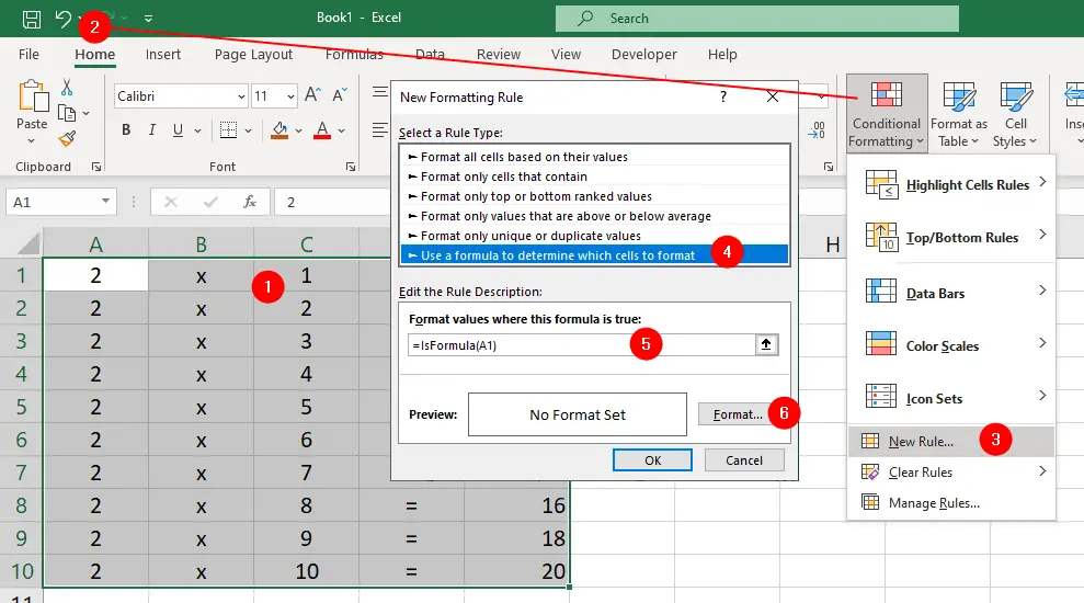
- Select a range of cells on your spreadsheet, e.g.
A1:J50.
Avoid the temptation of selecting an entire worksheet, as this can add unnecessary overhead to your spreadsheet. - With these cells selected, and with
A1the active cell of the selection, go to theHometab, in theStylesgroup, and clickConditional Formatting. - Click
New Rule. - In the New Formatting Rule dialog box, select
Use a formula to determine which cells to format. - In the
Format values where this formula is truebox, enter=ISFORMULA(A1), whereA1is the first cell in your selected range. - Click the
Formatbutton and choose any formatting you want to use to identify formula cells. - Click OK, then OK again.
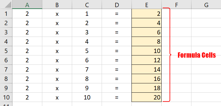
At this point, the specified formula should be applied to all cells on your worksheet that contain formulas. If you delete or overtype a cell containing a formula, the conditional formatting will disappear. Similarly, if you enter a new formula into any cell within the range, it too will be highlighted.

This simple conditional formatting can make your spreadsheets a lot easier to deal with when it comes time to maintain or modify them.
IsFormula Function Returns #NAME! Error
This error occurs when Excel does not recognize the function name or the syntax of the formula. To fix this error, you need to make sure that the function name is spelled correctly, and that the formula follows the proper syntax rules.
This function is available in Excel 2013 and later versions. If you use this function in earlier versions of Excel, you may encounter compatibility issues, such as #VALUE! or #NAME! errors. To avoid these issues, you can use the VBA code in this custom function (also called a user-defined function).
Creating IsFormula Function (User Defined Function)
Previous Excel versions do not have a built-in function that identifies formulas. Once a formula is entered into a cell, you can tell whether the cell is a static value or a value derived from a formula only by clicking on each cell and looking in the Formula bar. This tutorial fills that gap with a custom function.
The VBA code in this custom function (also called a user-defined function) enables you to identify cells that contain formulas without having to click through 10,000 cells and examine each one.

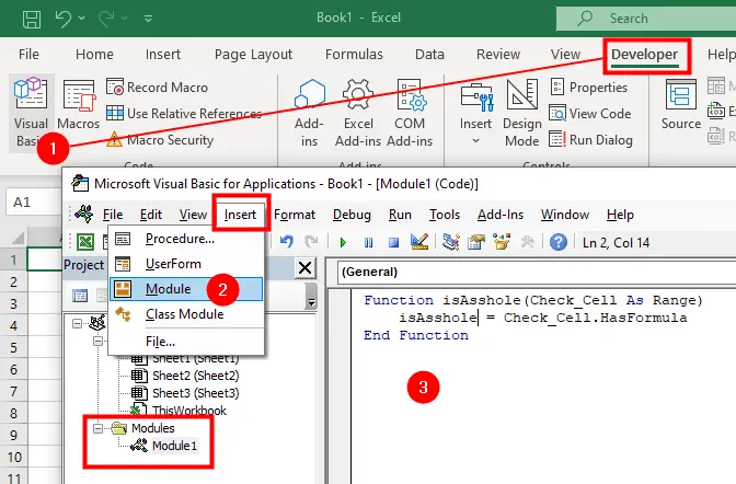
- Press
Alt+F11(orOptions+F11) to open Visual Basic Editor. - Click
Insert > Module. - Enter the following function:
Function IsFormula(Check_Cell As Range)
    IsFormula = Check_Cell.HasFormula
End Function
Close the window. Now this function is available in any cell on any worksheet in this workbook when you enter the formula =IsFormula($A$1).
You can also use conditional formatting to highlight formula cells in a different color, font, or border style as we described earlier in this tutorial.
Conditional Formatting
- Setting Up Checkboxes for Conditional Formatting
- Highlighting Formula Cells with Conditional Formatting
- Sum Cells That Meet Conditional Formatting Criteria
- Highlight Every Other Row or Column with MOD Function and Conditional Formatting
- Enable and Disable Conditional Formatting with a Checkbox
- Sort Data By Conditional Formatting Criteria
