Spill Range
Spill range is a term that refers to the range of values that a dynamic array formula produces and outputs onto the worksheet. The spill range is marked by a blue border and only the top-left cell contains the formula.
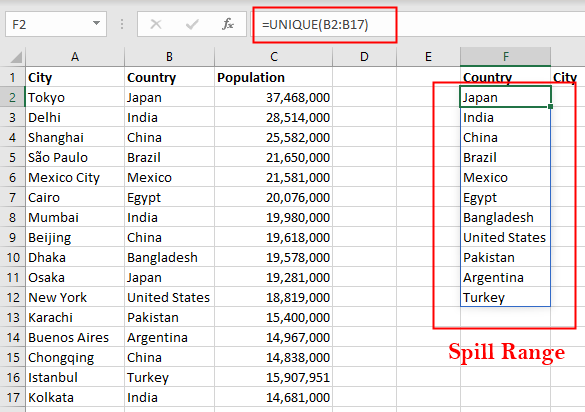
The spill range is dynamic and updates automatically as the source data changes. To refer to a whole spill range, you can use the spilled range operator (#) after the address of the upper left cell in the range. For example, if you have a UNIQUE formula in F2 cell that returns multiple values, you can reference all those values by typing =F2#.
Creating a Unique Drop-Down List with Spill Range
Dynamic array formulas allow you to work with multiple values at the same time in a single formula. However, dynamic array formulas cannot be used directly in a Data Validation rule. So, in this example, we have used the UNIQUE function in cell F2 to extract unique values from a cell range.
This formula returns a spill range of unique country names, which appear in F2:F12. Using the # symbol, we can then reference this spill range from the Data Validation dialog box. Follow these steps to create a Data Validation Drop-List From a Spill Range:
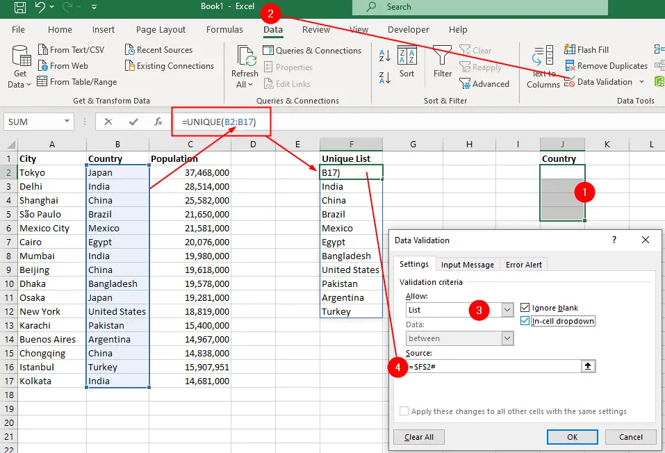
- Select the cell or range of cells you want to apply data validation to. I’ve selected
J2:J5. - Go to
Data > Data Validation. - Select
ListfromAllowoption in the Settings tab. - In the
Sourcebox enter$F$2#. - Click
OK.
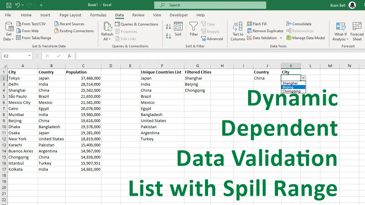
Creating Dependent Drop-Down List With Spill Range
We used UNIQUE function to create our first drop-down list with spill range. To create a dependent list with a spill range based on the selection of the first drop-down we’ll use FILTER function.
The FILTER function allows you to extract data from a range based on the criteria that you specify. The function has three arguments:
- array – the range or array that you want to filter.
- include – defines the criteria for filtering
- if_empty – (optional) value that you can provide to display when there are no matching results.
We want to filter a range (A2:A17) of cities data and only show the records (cities) where the country (B2:B17) is selected in the drop-down cell on (J2), you can use this formula:
=FILTER(A2:A17,B2:B17=J2,"Country is not selected.")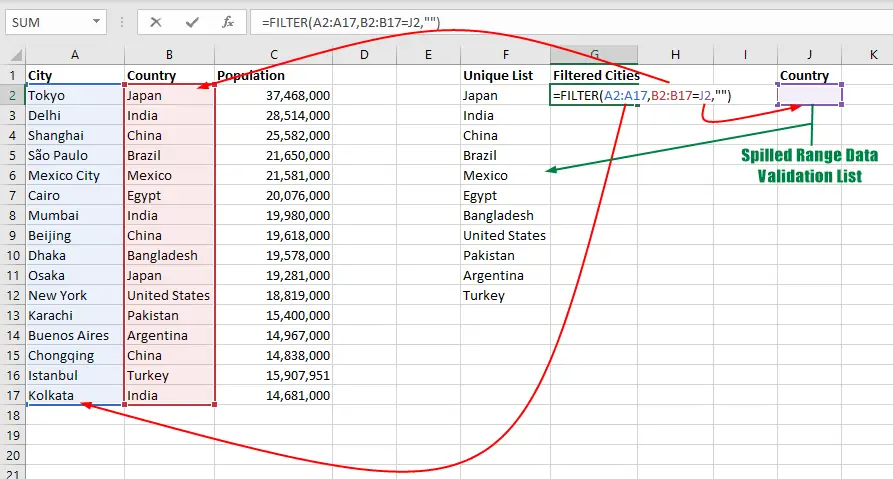
In our scenario, City data is in column A and Country data is in column B. We want to create another drop-down list that shows cities of the selected country in the drop-down on J2 cell. To do this, first, we use the FILTER formula like =FILTER(A2:A17,B2:B17=J2,"") in cell G2. This will create a spill range in column G that shows only the cities of the country that is selected in the J2 cell data validation list.
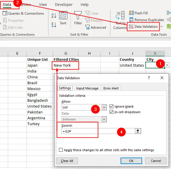
Then, we apply the data validation in cell K2 and set the source to =G2#. This way, whenever you change the country in J2, the dependent drop-down in cell K2 list will automatically update to reflect the changes.
Follow this link to watch how the dependent validation lists with spill range work.