Create Validation Lists That Change Based on a Selection from Another List
Prepare the source data for the lists. You need to have a column (or row) with the main categories, and another column (or row) with the types that correspond to each category. Make sure the categories have unique names.
To create a cascading data validation list, you first need to create a drop-down list for the main categories:
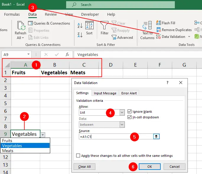
- To create a drop-down list, you need to prepare a range of cells with the list items. The range can be either one row or one column. The drop-down list will display the items from the range you specify.
- Click on the cell where you want the list to appear.
- Go to the
Datatab and click onData Validationin the Data Tools group. - Select
Listfrom theAllowoption from the Settings tab in the Data Validation dialog box. - In the
Sourcebox, specify the range that contains the list. The range can be in a different worksheet. - Click OK.
Creating Dependent List
Now you need to create another drop-down list (subcategories) that changes based on the value selected in the (categories) previous drop-down list:
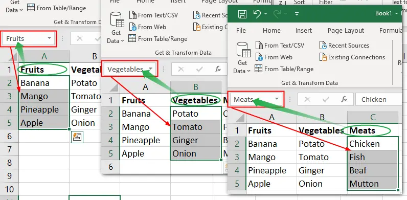
- Create named ranges for each category. You can use the Name Box to define names for each dependent list (subcategories).
- The names of the dependent lists should match exactly with the names of the categories.
For example, suppose you have a list of fruit names in a certain range of cells. You can assign the name Fruits to this range by typing it in the Name Box as this match exactly with one of the name of the category.
- Select the cell where you want the second drop-down list to appear.
- Go to
Data > Data Validation. - Choose
Listas the Allow option - In the Source box enter this formula:
=INDIRECT($A$9), whereA9is the cell with the second drop-down list. - Click OK.
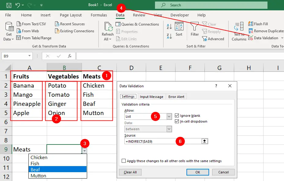
Test your cascading data validation list. Select a value from the first drop-down list, and see how the second drop-down list changes accordingly.