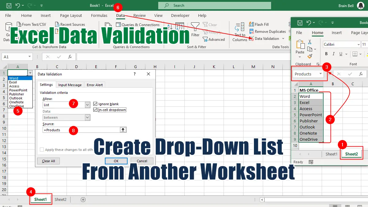
In this tutorial, we will show you how to create a drop-down list from another worksheet in Excel.
- Create a list of values on another worksheet
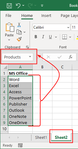
The first step is to create a list of values on another worksheet that you want to use as your data validation source. For example, a list of items onSheet2that you want to use in other sheets e.g. Sheet1, Sheet3, etc. - Name the list of values
Select the cells of the list, click the Name box, on the left of the Formula Bar, and type the name that you’ll be using to refer to the list, then press Enter.

Named ranges are unique in a Workbook and can be accessed from any worksheet in the Workbook without requiring you to enter the sheet name.
For example, if you have a named range called “Sales” in Sheet1, you can use =SUM(Sales) in Sheet2 (or in any other sheet) without specifying Sheet1!Sales.
- Apply data validation to the target cells

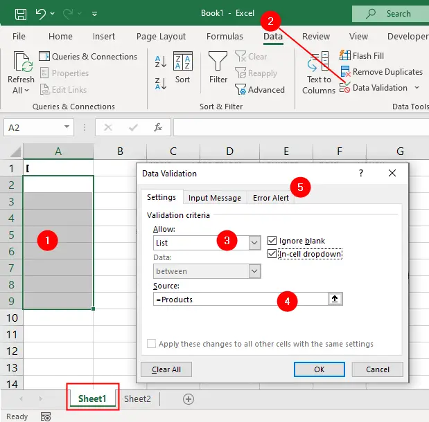
The final step is to apply data validation to the cells where you want to use the drop-down list from another worksheet. To do this:
- Select the target cells
- Click
Data > Data Validation. - In the Data Validation dialog box, choose
Listfrom theAllowoption - In the
Sourcebox enter the name of the list you created inSheet2by an equal sign, for example,=Products. - Make sure the
In-celldropdown option is checked. - Click OK.

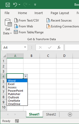
Now you have a drop-down list from another worksheet that you can use to enter data in your target cells. You can also update the source list on Sheet2 and see the changes reflected in the drop-down list on Sheet1.
