There are several ways to update a chart in Excel:
- You can manually enter or edit data in the chart’s data range, and the chart will automatically update to reflect the changes.
- Use a dynamic range for your chart data (e.g., using Excel tables or named ranges), any changes or additions to the data within the defined range will automatically update the chart. Visit following posts:
- You can directly edit the chart itself by right-clicking on elements of the chart (like data series, axes, titles, etc.) and selecting options to modify them. This doesn’t update the data but allows you to customize the appearance of the chart.
- Use the
SERIESfunction to create or modify a series within a chart. It is often used in conjunction with other chart-related functions to customize the appearance and behavior of chart elements.
The SERIES Function
You can update your chart by using the Formula bar. When you select a chart and click a data series within it, look at the Formula bar and you will see the SERIES formula Excel uses for the data series.
The formula generally uses four arguments, although a bubble chart requires an additional fifth argument for [Size].
The syntax (or order of structure) of the SERIES function is as follows:
=SERIES( [Name] , [X Values] , [Y Values] , [Plot Order] )So, a valid SERIES function could appear as follows, and as shown in figure:
=SERIES(Sheet1!$B$1,Sheet1!$A$2:$A$6,Sheet1!$B$2:$B$6,1)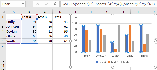
In terms of Figure:
- The first part of the reference,
Sheet1!$B$1, refers to the name, or the series title, which is Test A. - The second part of the reference,
Sheet1!$A$2:$A$6, refers to the X values, which in this case are the Names. - The third part of the reference,
Sheet1!$B$2:$B$6, refers to the Y values, which are the values 91, 94, 35, 60, and 94. - The last part of the formula, the
1, refers to the plot order, or the order of the series. The first series would take the number1, the second series would take the number2, and so forth.
To make changes to the chart, simply alter the cell references in the Formula bar.