Starting with some data such as that shown in the following figure, you will add a dynamic range that will be used as a data source for the chart.
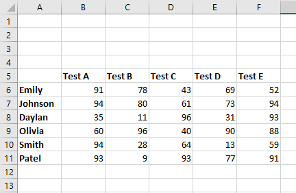
The dynamic range will be linked to a drop-down list you can use to view one student’s test results from those of a group of students. You will use the drop-down list to select the name of the student whose results you want to view.
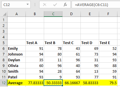
Use the formula =AVERAGE(B6:B11) in cell B12 and copy it across to cell F12, as shown in the figure:
Create Dynamic Ranges
Create a dynamic range by selecting Formulas » Define Name, and call it STUDENTS. In the Refers To: box, type the following:
=OFFSET($A$5,$G$6,1,1,5)
Create another dynamic range called STUDENT_NAME, and in the Refers To: box, type the following:
=OFFSET($A$5,$G$6,0,1,1)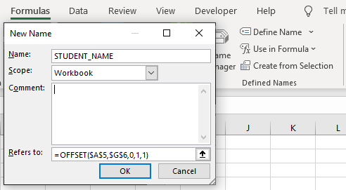
The use of the cell reference $G$6 in the OFFSET formula forces the referenced ranges for STUDENTS and STUDENT_NAME to expand both up and down as the number in $G$6 changes.
Create Clustered Column Chart
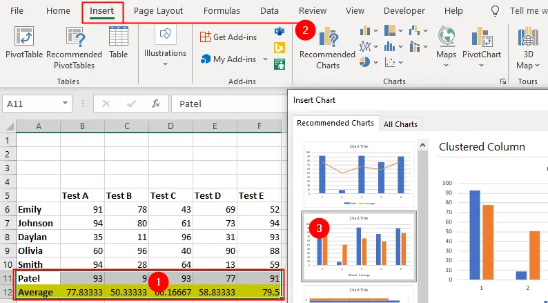
Now create a clustered column chart using the range A11:F12 as shown in the figure above.
Next, edit the chart data to use the dynamic named ranges:
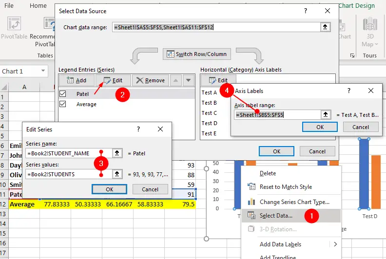
- Right click on the chart and click
Select Datafrom the context menu. The Select Data Source dialog box will be displayed. - Select the first series (
Patel) from the Legend Entries (Series) tab and clickEditbutton. - In the Edit Series box:
- Enter
Workbook_name!STUDENT_NAMEin the theSeries name:box. - Enter
Workbook_name!STUDENTSin theSeries valuesbox. - Click OK to close the Edit Series box.
- Enter
- Now, click the
Editbutton from the Horizontal (Category) Axis Labels tab and select the top headingB5:F5and press OK.
Inserting Combo Box
At this point, you need to insert a Combo Box from the Forms Controls:
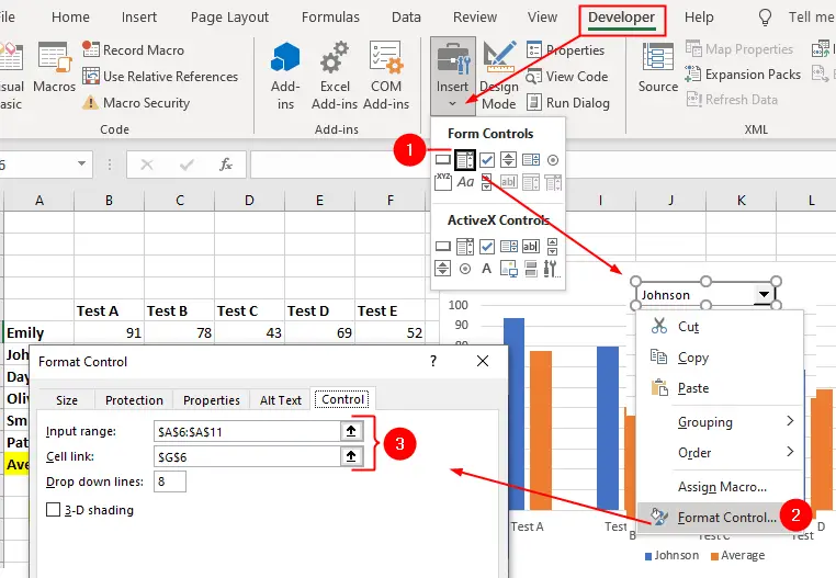
- Go to the
Developertab and select the Combo Box icon from the Insert drop-down menu to insert it on the sheet. - Right-click on the combo box and choose
Format Controlfrom the context menu. - Enter
$A$6:$A$11for the input range and enter$G$6for the cell link. - Click OK.
Clicking the downward-pointing arrow on the Combo Box shown in the figure will change the name of the student and show his test results: