As you saw in the Use Dynamic Named Ranges to Create Charts tutorial, you can use dynamic named ranges to add flexibility to your charts. But you also can use dynamic named ranges to create interfaces controlling which data the chart plots. By linking dynamic named ranges to custom controls, you enable users to change the chart data by using the control, which simultaneously will update the data in the worksheet or vice versa.
Using a Dynamic Named Range Linked to a Scrollbar
- Insert Chart
- Create Dynamic Named Range
- Insert Scroll Bar
- Change chart’s data source to use named range created on step 2
In this example, you will use a scrollbar to reveal monthly figures over a 12-month period. The scrollbar is used to alter the number of months reported. The scrollbar’s value also is used in a dynamic range, which in turn is used as the data source of the chart.
Insert Chart
To begin, insert a bar or line chart using some data similar to that shown in the figure:
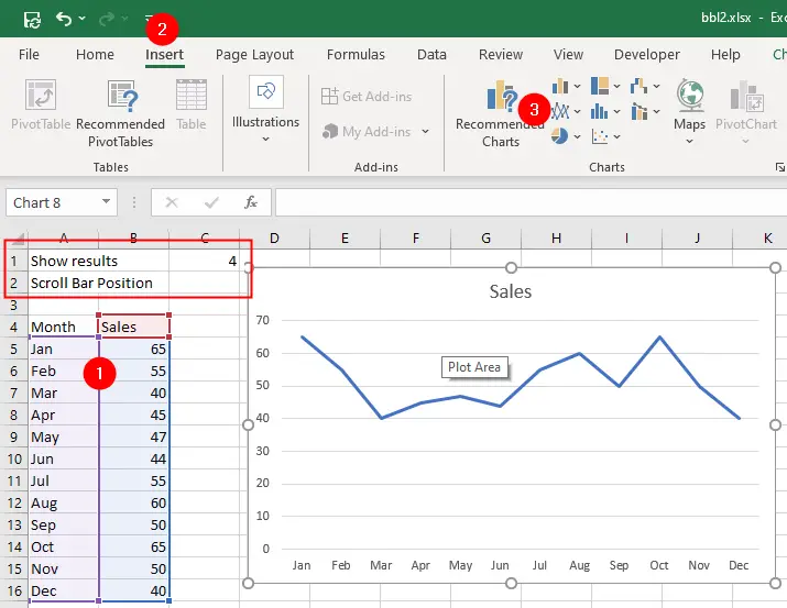
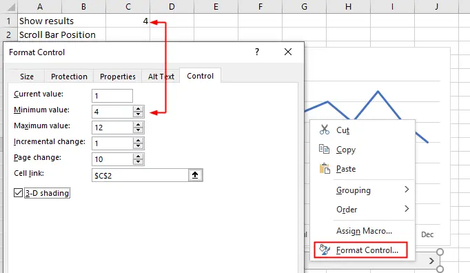
The value entered in cell C1, labeled ‘Show results,’ dictates the number of records displayed on the chart.
The cell C2, labeled ‘Scroll Bar Position’, will be linked to the scroll bar.
2. Create Dynamic Named Ranges
Next, create a dynamic named range by selecting Formulas » Define Name and call it SALES_PERIOD.
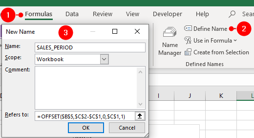
In the Refers To: box, type the following:
=OFFSET($B$5,$C$2-$C$1,0,$C$1,1)By using the OFFSET function, you can use cells $C$1 and $C$2 to force the referenced range for SALES_PERIOD to expand both up and down as the number in $C$2 changes when the scroll bar moves. In other words, changing the number in $C$2 to the number 5 would force the range to incorporate B5:B10.
Let’s dissect the =OFFSET($B$5, $C$2-$C$1, 0, $C$1, 1) formula step by step:
$B$5: This is the starting reference point, referring to cell B5.$C$2-$C$1: This part calculates the number of rows to move down from the starting reference point. It subtracts the value in cell C1 from the value in cell C2 (scrollbar position). This calculation may result in moving the reference point up or down depending on the relative values of C1 and C2.0: This parameter specifies the number of columns to move horizontally from the starting reference point. Since it’s 0, it means the reference point remains in the same column.$C$1: This parameter specifies the height of the range. It’s referencing the value in cell C1, which likely indicates the number of rows you want in the output range.1: This parameter specifies the width of the range. It’s set to 1, so the output range will be one column wide.
Make Horizontal (Category) Axis Scrollable
Next, create another dynamic named range by selecting Formulas » Define Name and call it H_AXIS_PERIOD. In the Refers To: box, type the following:
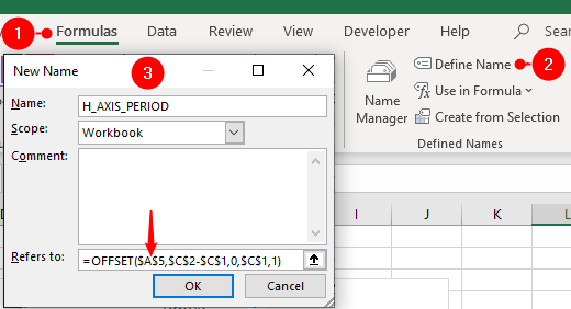
=OFFSET($A$5,$C$2-$C$1,0,$C$1,1)This formula works similar to the previous formula, we just change the the starting reference point to A5.
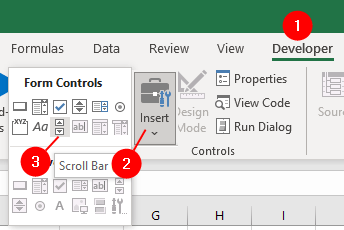
3. Insert Scroll Bar
Click Developer tab and in the Controls group click Insert drop-down and select the scrollbar icon to insert a scrollbar:
Once you have inserted a scrollbar, select it and move it onto your chart. Now right-click it and select Format Control, change the minimum value to value you entered in cell C1 (for example, write 4 if you’ve entered 4 in cell C1), change the maximum value to 12, and set the cell link to $C$2:
4. Change The Data Series
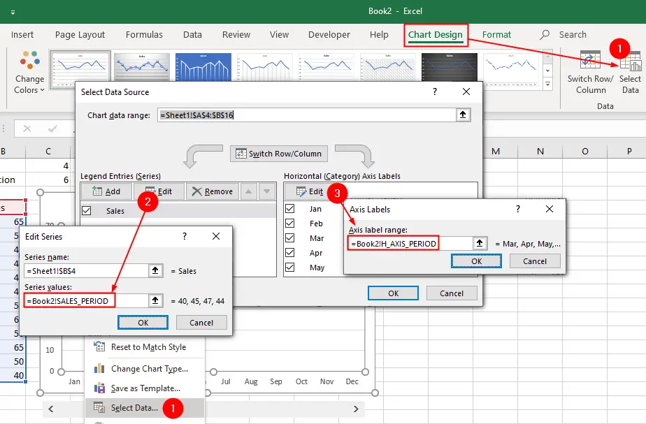
- Next, right click on the chart and click
Select Data, the “Select Data Source” dialog box will be opened. - In the Legend Entries (Series) tab click the
Editbutton to open the “Edit Series” dialog box.
In the Series values: box write=WORKBOOK_NAME!SALES_PERIOD.
Click OK. - In the Horizontal (Category) Axis Labels tab, click the
Editbutton to open the Axis Labels dialog box.
In the Axis label range: box write=WORKBOOK_NAME!H_AXIS_PERIOD.
Click OK. - Click OK again to close the “Select Data Source” dialog box.
Doing this will make your chart dynamic. The resulting chart will look like that shown in the above figure.