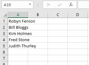
Assume you have a list of names in the range A1:A5, as in the figure:

These names represent employees in a company. It is not uncommon for new employees to be added to such a list, but the only way to achieve this is to add the new names to the end of the list and then select the new names from the list in the validated cell.
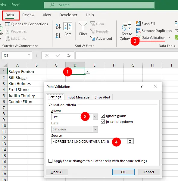
To overcome this limitation, you can use the following formula in the data validation rule:
=OFFSET($A$1,0,0,COUNTA($A:$A),1)- Select the cells where you want to apply the data validation rule.
- Go to
Data > Data Validation. - In the Data Validation dialog box, choose
Listfrom theAllowdrop-down menu. - In the
Sourcebox, enter the formula=OFFSET($A$1,0,0,COUNTA($A:$A),1). - Click
OKto apply the data validation rule.

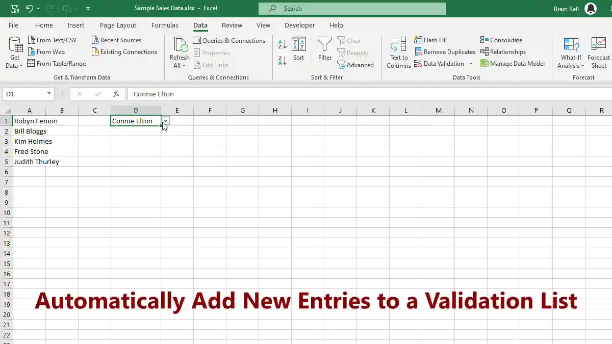
Now, whenever you add a new item to the list in column A, it will automatically appear in the validation list in the other cells.
The formula =OFFSET($A$1,0,0,COUNTA($A:$A),1) is used to create a dynamic range that expands or contracts based on the number of non-empty cells in column A. The formula works as follows:
- The first argument,
$A$1, is the reference cell that defines the starting point of the range. - The second and third arguments,
0and0, are the offsets in rows and columns from the reference cell. In this case, they are both zero, meaning the range starts at$A$1. - The fourth argument,
COUNTA($A:$A), is the height of the range in rows. It counts how many cells in columnAhave any value, and returns that number as the height of the range. - The fifth argument,
1, is the width of the range in columns. It is fixed at1, meaning the range only covers one column (columnA).
The formula returns a range that starts at $A$1 and ends at the last non-empty cell in column A. This range can be used as a source for data validation lists that require a dynamic range.
